•  
    Living Paper: An Open Source Project


    Proposed Economics Programs

    1. Curvedraw.ý

    2. Budget Line Indifference Curve Draw.ý .

    3. Demand Supply Monopoly. ý .

    4. Edgeworth box. Program 2 + 2nd I curve, axes, coordinates.

    5. The Invisible World&endash; S/D Identification problem game. *

    6. Elasticity, TR, MR.*

    7. ¹ maximize in two markets; discover MR1=MR2.

    8. Supermarket seen from above&endash;lines.*

    9. Price control, line, D shifted, surplus.

    10. Disneyland ride lines&endash;like 9 + 2 part pricing + ¹ maximizing.

    11. Highway congestion, peak load pricing, seen from above.

    12. Tariffs, exchange rates, surplus; design efficient tariff.

    13. Linked markets transmitting&endash;labor or crops.

    14. Central planning trade game with comparative advantage.

    15. Arbitrage game: Sij curves. Trade converges relative prices.*

    16. Sunk Cost game: Random walk P, invest, produce.

    17. Experimental monopolist&endash;searching for D.

    18. [Cartel game: Abide or chisel? Probabilistic monitoring.]

    19. [Programmed oligopolist].

    20. Tax and Welfare&endash;The fundamental dilemma.

    21. N dimensional economics.

    22. Joint Product Game.

    23. Monopoly II: How To Lose Your Shirt.

    24. Present Value Visual Calculator*

    25. Cleaning Out Cobwebs: Speculation vs the Hog/Corn cycle*

    26. Experimental game theory

    27. Hansa.*


    Macro

    28. Nail Something Down (Macro).

    29. Milton Keynes

    ý Versions of these programs exist as part of the collection of programs accompanying Price Theory: An Intermediate Text, by David Friedman. They are subject to contractual agreements with South-Western. New programs along similar lines will be part of the collection described here.

    *: Detailed description exists.


    Short Program Descriptions


    1. Curvedraw. Mark II.

    Student draws TC, AC, or MC; computer simultaneously draws one or both of the others. If the student is drawing the function and the computer the integral, there is the option of showing the shaded area under the funciton. If vice-versa, option of showing the tangent line. Also, can click on either line and get tangent or area accordingly. Can be used for calculus review as well as cost etc.


    2. Budget Line Indifference Curve Draw.

    A set of tools for doing general budget line-indifference curve diagrams.

    (2 Dimensional economics--includes labor leisure, 2 input isocost/isoquant. Add tool to show MRS, MRT.)


    3. Demand Supply Monopoly.

    Student calculates demand curve from marginal revenue curve, supply curve from marginal cost.Student finds profit maximizing monopoly price, checks that it is where MR=MC.


    4. Edgeworth box.

    This is like program 2, with two individuals. "Gravity field" driving to contract curve as option?


    5. The Invisible World

    Student picks one of N commodities, adjust 3 variables to affect supply and demand curves. Only P,Q at equilibrium is shown. Student deduces D, S, replays with curves visible to see what he did.


    6. Elasticity, TR, MR.

    Student draws a demand curve. Program shows elasticity at any point, TR and MR at request.


    7. ¹ maximize in two markets.

    Works like monopoly part of 3; student discovers MR1=MR2 rule.


    8. Supermarket Seen from above.

    Student controls the parameters, watches the equilibrium.


    9. Price control, line.

    Student sets the controlled price, program shows line forming, effect on waiting of value to consumer (D shifts down), surplus as area and number, profit.


    10. Disneyland ride lines

    Like 9 + 2 part pricing + ¹ maximizing.


    11. Highway congestion, peak load pricing.

    Demand curve shifts by time of day, falls as travel time increases. Student sets price schedule, watches the result.


    12. Tariffs, exchange rates.

    Two goods, two countries, supply and demand curves can be varied. Student adjusts tariff (± ) and export tax (± ) to maximize net benefit, watching exchange rate and flow of goods adjust.


    13. Linked markets transmitting.

    A set of markets, such as different crops or different professions, linked by common inputs. Change demand in one market and watch the effect.


    14. Central planning trade game.

    The student controls several factories. Each has a fixed amount of labor available per week, and output rates/unit labor for different goods. Each also has its own market with demand curves. Factories can sell locally or export with a small transport cost. Student tries to maximize his profits. He discovers "trade" based on comparative advantage.


    15. Arbitrage game:

    There exist net supply curves Sij for trading any pair of goods i,j. student starts with fixed amount of a good, tries to increase his holdings by arbitrage. Ideally, 2 or more students play at once; best arbitrageur finds the opportunities first and eliminates them while profiting from them.


    16. Sunk Cost game.

    Price is a random walk, student invests and produces to maximize his profit.


    17. Experimental monopolist.

    Student is a single price monopoly who initially does not know his demand curve. Experimental pricing to find profit maximizing price. Could also do it with two markets.


    18. [Cartel game: Abide or chisel? Probabilistic monitoring.]

    19. [Programmed oligopolist].


    20. Tax and Welfare&endash;The fundamental dilemma.

    Student tries to adjust marginal rates, positive and negative, implied by a system of taxes and welfare, while being held to a budget constraint; program specifies (or student chooses) elasticities of labor supply and tax evasion. Program calculates gini coefficient.


    21. N dimensional economics. Maximize utility while consuming n=3-5 goods. Maximize output with n inputs. Like production in Hanse, but transfer a dollar's worth per click when you link two scroll bars (two goods). Show dollar's worth, MU (or MP).


    22. Joint Product Game. You face demand curves (perhaps perfectly elastic) for two goods, joint cost, separable cost. Maximize profit.


    23. Monopoly II: How To Lose Your Shirt. Game version of predatory pricing argument?


    24. Present Value Visual Calculator. The student finds the present value of a series of payments in a way that visually shows how the present value of a dollar shrinks the farther in the future it is received.*


    25. Cleaning Out Cobwebs: Speculation vs the Hog/Corn cycle. Draw a demand and supply curve, generate a cobweb, show as graphs of P and Q against time. Add speculators to the market, give them buy/sell rule, and watch the graph smooth.*


    26. Experimental game theory: A program to apply Axelrod’s approach to several games. Prisoner’s dilemma, Bilateral monopoly, 3 player majority vote, scissors/paper/stone. ...?


    27. Hanse.*

    Game of building up a trade league.


    Macro Programs


    28. Nail Something Down (Macro). Fix one variable, watch the rest adjust. Fix price, get Keynesian Cross. Fix income, get quantity theory. Fix ???


    29: Milton Keynes.

    Student is the economic Czar. The economy is either simple Keynesian or simple Monetarist; initially student does not know which. By manipulating deficits, money supply, etc. student affects economic outcomes, trying to maximize some measure of economic welfare.


    General Comments


    These programs are intended as a package to be used in economics courses at the principles and intermediate level. There are two ways in which they might be marketed&endash;separately or as a tie-in with particular texts. In the following discussion, I will assume the latter.


    Customization


    The package could be customized to a particular textbook in any or all of three different ways. First, one could select those programs appropriate to the text. Second, the instruction files built into each program could be modified, possibly by the textbook's author, to include specific references to points made in his book, chapter titles, page numbers, problems, etc.


    In some of the descriptions, I suggest alternative ways in which the program could be written; typically some are harder than others. Demand and supply curves, for instance, could be restricted to straight lines, or permitted to be curves. Price and quantity might be observed with precision, or with some error. In some cases the program should provide several different levels and allow the student to choose among them. In some cases we may decide, after testing the program, that one variant is unambiguously inferior to another and should be eliminated. In some cases we may use variant programs as a third way of customizing the package to a particular text. Thus, for a low level text, we might use straight lines and certainty where, for a higher level book, we would use curves and random errors.


    Choice of Computer


    Throughout these description I assume that the program is to be implemented on a Macintosh. An implementation under OS/2 and the presentation manager or under MSDos and Windows would be similar, with perhaps some use of color. Implementation under MSDos without windows or a mouse but with graphics would be possible but clumsier; cursor control keys would have to be used to draw curves, set values for variables, etc. Implementation on an MSDos machine with no graphics would not be worth doing.


    One reason to develop the programs first on a Macintosh is the lack of a dominant graphics standard in the MSDos world. At present, the only graphics common enough to matter for our purposes is CGA, and its quality is no more than minimally acceptable. In another year or two it may be possible to judge whether EGA, PGA, or VGA will be the dominant standard in the future, and whether we can count on students having access to machines runnings Windows or Presentation Manager and equipped with mice.


    Common Features


    The descriptions are intended to explain the special features of the different programs. In addition, there are some features which would be common to many or all of them. These include on-line help files of several sorts, and the ability to save, load, and print work in progress.


    Help


    Whenever one of the programs is being used, the student should have access to on-line help files. These would be of at least three kinds, which I will call Information, Help, and Projects. Information would be a description of the entire program&endash;what it does and how it works. Help would be specific context-sensitive information&endash;what the student is supposed to do at this point in the program. Projects would be a list of things to do with the program&endash;questions to learn the answer to, problems to solve.


    For the Macintosh, there exists a sophisticated help facility of this sort which can be licensed inexpensively; it might make sense to use that rather than writing our own. I do not know if similar things exist for MSDos machines. Ideally we want a system that makes it easy for us to modify the help files but hard for the user to do so; we do not want students adding their own comments to the instructions. We might, however, want to add an additional facility specifically for comments, in the form of a mini-word processor that could generate comments and questions for the professor to answer or bug reports to be sent to us.


    File Menu


    A student should be able to quit work at any time and resume later. All programs should therefore be equipped with a save command that saves the current status to disk and a load command that restores the program to its saved status. In addition many programs can generate graphical output and should therefore have a print command.


    There might be cases where it would be useful to transfer something, such as a demand curve, from one program to another. For instance, a student who had estimated the demand curve for program 17 (Experimental Monopolist) might want to examine its elasticity using program 6 (Elasticity, TR, MR). If so, we might want to use the Macintosh clipboard to move the curve from one program to the other. I am not certain this is worth the trouble of implementing, nor if it is exactly how it should be implemented, but it is at least worth considering.


    The Invisible World


    Student picks one of N commodities, picks values for several variables that affect supply and demand curves. Only P,Q at equilibrium is shown. Student deduces D, S, then replays to see what he did.


    Lesson


    In an economics course, students are repeatedly shown supply and demand curves. In the real world, one observes not the supply curve or the demand curve but the point where the two cross&endash;the equilibrium price and quantity. One cannot simply deduce the curves from looking at a lot of such points at different times or places, since the fact that price and/or quantity is different in year two than in year one implies that at least one of the curves is also different.


    To deduce a supply curve, one must look at a set of different points which one has some reason to believe are produced by one supply curve but several different demand curves. Since the points are all intersections they all lie on the supply curve and thus show its shape. Similarly, mutatis mutandis, for deducing a demand curve. Conceptually, the technique is equivalent to the method of instrumental variables in statistics.


    Program


    The student is shown a blank graph with quantity of a named commodity (say wool) on one axis and price on the other, and a list of three variables, such as weather, fashion, and meat prices. The variables are chosen in such a way that it is plausible that one affects the supply of the commodity (meat prices affect the supply of wool, since wool and lamb are joint products), one the demand (fashion), and the other one or two affect one, both, or neither (weather might affect both supply and demand, for instance).


    When the game starts, the program shows initial values for the variables and a point on the graph, labelled A, representing the intersection of the (invisible) supply and demand curves implied by those values. The student may alter the values and ask to see the new point produced by the new values; it will be labelled B. The student continues up to some maximum number of points. As he proceeds the screen shows the labelled points on the graph and also a list of values of the variables for each point (see screen below). Variables may have numerical values (prices of meat) or verbal values (weather might be good, fair, bad, cold, hot).


    The student starts with a score of 100, shown on the screen. Each point he asks to see beyond the first lowers his score by 5 points.


  •  


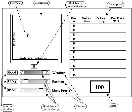
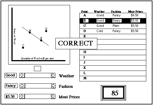
  • The next figure shows the screen after the student has just set his fourth point, D. The list of points shows the values for points A-D; the points themselves are shown on the drawing area. Note that the button above the scroll bars for the variables is labelled E, since clicking on it will draw the next point. If the student clicked E without changing the values of any of the variables, E would appear on top of D.
  •  


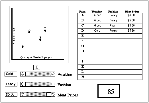
  • When the student believes that he has enough points (or when he has done as many as the program permits), he draws a supply curve and a demand curve, specifying the values of the variables for which each applies. The drawing is done with a mouse (Macintosh version); the specifying is done by clicking on the line on the list of values corresponding to one of his points. The program tells him if he is correct. If not, and if he has not used the maximum permitted number of points, he may get additional points before trying again. Each incorrect try lowers his score by 10 points. The figure below shows the screen just after the student has correctly drawn the demand curve corresponding to point B.


    When the student has either successfully drawn a supply curve and a demand curve or used up all his points and given up, he is given a score (higher the fewer points used and the fewer wrong tries&endash;0 if he never gets either curve right) and an opportunity to watch a "replay."


  •  


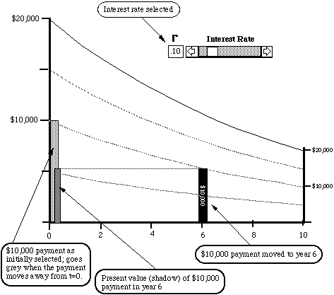
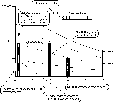
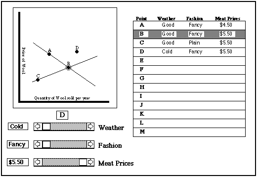
  • The replay starts with the values of the variables corresponding to point A. This time, the supply and demand curve are shown on the screen, along with their intersection (at point A). If the student clicks on any other point (either a labelled point or the corresponding line in the list of values) the screen shows the supply and demand curves for that point. The figure below shows the situation after the student has clicked on point B.


    Bells and Whistles


    There are several additional features that might be added. So far I have assumed that supply and demand curves are straight lines. The student could be given the option of permitting the program to use smooth curves as well.


    A more interesting change would be to permit supply and demand curves to be influenced by additional factors not controlled by the student. The simplest way would be to add a small random term. The student, in drawing the curve, would be engaged not in rigorous deduction but statistical inference&endash;although the random term would be small enough so that the statistics could be done by eye. Alternatively, one might add an additional variable which the student could observe but not control, and which would vary randomly. If so, the variable should affect supply or demand but not both; that way a clever student could find one set of curves and use that knowledge in approximating the other.


    A student selecting either of these "higher level" versions would start with a larger number of points and thus get a higher score for any given number of points chosen and errors made.


  •  


  • In my description so far, I have considered only one good, wool. The program should have a built-in list of ten or twenty goods, each with its corresponding variables and each variable with its corresponding list of possible values. The player starts by choosing a good, probably by scrolling through a list and double clicking on one; alternatively the program might choose one for him at random. In any case, the parameters of the actual curves should be chosen randomly each time the game is played.


    I have assumed that the number of points the player is permitted to choose is limited to the number that will fit on the on-screen list. Alternatively, the list could be scrollable, permitting an unlimited number of points. One argument against this is that with more than a dozen or so points the drawing area may get pretty crowded.


    There are a number of details of the program that I have not described, such as how the student tells the program that he is ready to draw curves. That might be a menu choice or an on-screen button. I have not described how the student actually draws a curve. If all curves are straight lines, one could use something like the line-drawing tool in MacDraw, which allows you to draw a line with the mouse and then move its end points around until it is properly located.


    Mathematics


    The underlying mathematics of the program are simple. We have a supply curve:


    Qs=As+Bs*P


    And a demand curve:


    Qd=Ad-Bd*P


    Each time the program is run or a new commodity is selected, values are randomly chosen for the parameters of the curves. In addition, the parameters are functions of the variables, with (as mentioned above) the supply parameters depending on one variable, the demand parameters on another, and a third variable entering one or both sets. All values of the parameters must obey the conditions:


    1<Bs<5; 1<Bd<5 Condition 1


    (200-200*Bs)<As<0; 200<Ad<200*Bd Condition 2


    Ad/Bd>-As/Bs; (Ad-200)/Bd<(200-As)/Bs Condition 3


    Here the units for price and quantity are pixels; the drawing area is assumed to be 200x200, roughly corresponding to the figures. Conditions 1 and 2 guarantee that the supply and demand curves will be entirely in the drawing area&endash;or in other words, that if Q is between 0 and 200 so is P. Condition 3 guarantees that the demand curve is above the supply curve for Q=0 and below for Q_=200, and thus that the two intersect for some 0<Q<200.


    Once the parameters are determined (by an initial random procedure plus the effect of the values choosen for the variables) the program solves for Qs=Qd to find the point.


    Arbitrage game


    There exist net supply curves Sij for trading any pair of goods i,j. Student starts with fixed amount of a good, tries to increase his holdings by arbitrage. Ideally, 2 or more students play at once; best arbitrageur finds the opportunities first and eliminates them while profiting from them.


    The Lesson


    Goods exchange for other goods; at any instant there is a price at which good i can be exchanged for good j. These prices tend to be consistent; if one unit of i trades for two units of j, and one unit of j trades for 3 of k, then one unit of i will trade for about six units of k (pik@pijpjk).


    One reason for the consistency is that if the prices are not consistent (pik­ pijpjk) it is possible for someone to profit by a series of trades in which he goes one direction (say from i to k) indirectly (exchanges i for j and then j for k) and the other direction directly (exchanges k for i), ending up with more of his initial good (i) than he started with. One effect of such trades is to bid the low prices up and the high prices down, moving the set of prices towards consistency.


    The purpose of the program is to allow students to see how this mechanism works by themselves engaging in such trades (arbitrage).


    The Program


    There are two forms for the program, both of which will be described. The essential difference between them is in the equations determining prices. Either form may be played in either a one player or multiple player version; in the former the computer simulates the effect of additional arbitrageurs. The multiple player version could be played either on one machine or on several machines attached to a network. It should probably be designed for one machine and a network version created later if it looks as though networks are becoming sufficiently common to justify it. I will describe only the one machine version.


    Single Player


    There are five goods, hence ten prices (5x4/2). At the beginning, the program shows all ten prices and the amount of one commodity that the player starts with. Each turn the player trades some or all of what he has for one or more of the other goods; once the game has been going for a while he may have stocks of any or all of the five goods. Units acquired in one turn cannot be traded again until the next.


    Each turn, there is a new set of prices. The player chooses what trades to make; his stock of commodities is altered accordingly. After a fixed number of turns, the game ends. All stocks of any good he holds other than the good he started with are converted into that good at the then prevailing prices. His score is the ratio of the amount of that good he then has to the amount he started with.


    Multiple Player


    In the multiple player version players move consecutively; prices are recalculated after every move. Players begin by choosing an initial bundle&endash;a given amount of a given commodity&endash;from alternative bundles offered by the program. The player who chooses last moves first.


    Options


    In a more advanced version, the player is managing an arbitrage fund, with specific objectives. If he choose to manage a low risk fund, the computer fires him if the value of his holdings drop by more than a stated percentage in any turn. If he manages a high risk fund, he is judged only be increase at the end. Other variants could be constructed.


    New Ideas (1990)


    1. Playing in real time. Repeated plays, computer reports cumulative average.


    2. Player (or computer) chooses degree of risk aversion. Window shows utility as a function of income. If risk neutral, $1=1 utile. Again, computer reports cumulative average--this time utility as well as income.


    3. Use currency, show a table of prices each way.


    4. One can either have the underlying formula keep relative prices fixed, with random variation about that set of prices to introduce inconsistency, or one can allow relative prices to change substantially. In the second case, a player is exposed to substantial speculative risk. Diversification both allows safe arbitrage and reduces risk--sensible for risk averse players.


    Mathematics


    Version 1


    In this version of the game, trades made by the players have no effect on prices; it corresponds to a situation in which the individual arbitrageur controls a negligable fraction of the goods on the market. Prices are set randomly each turn, with some tendency to move towards consistent values.


    A simple way of modelling this would be for the program to randomly choose one good each turn, hold fixed the prices of the other goods in terms of that good, adjust all other prices towards consistency with those, then add in a random change to every price. The resulting equations, with i the good chosen randomly after turn t, would be:


      , "j­ i


     ,"j,k­ i; j­ k


    Here 0<a<1 is a parameter measuring the tendency towards consistency; the larger it is the more slowly inconsistencies in prices vanish. eij is a random variable.


    Version 2


    Underlying the game is a set of excess supply curves (quantity supplied minus quantity demanded as a function of price) representing net supply by non-arbitrageurs in each two good market. If, for instance, excess supply of oranges on the orange/apple market is -2 at a price of 1, that means that if one apple traded for one orange then the number of oranges offered by people who had oranges and wanted apples would be two fewer than the number of apples offered by people who wanted oranges and had apples. Since excess supply (including supply by arbitrageurs) must be zero at the equilibrium price (quantity supplied equals quantity demanded), price will be such as to make excess supply by non-arbitrageurs equal to demand by arbitrageurs.


    Part of the point of this version of the game is that a player, by seeing and exploiting an opportunity to profit by arbitrage, eliminates or reduces that opportunity for other players or himself on later moves. In order for this to be true, units sold in one turn must effect the market in future turns, either because some of them are stored and consumed later or because of intertemporal substitution.


    In the simplest form, we have a single period of production and consumption during which there are multiple periods of arbitrage. On each of the ten markets (ij), we have


    Here is the quantity demanded by arbitrageurs (players) in period t on the ij market&endash;or in other words, the number of units of j which players exchange units of i for. Aij is what the price would be on the ij market if there were no trades by arbitrageurs.


    Note that in this version of the game, the price faced by a player is a function of how much he wishes to trade. The interface, as described below, reflects this; as the player changes the amount of his planned trade the price he will get also changes.


    Two additional complications could be added to the underlying model. One is a random element; instead of A having a fixed value, we have:


    Aij(t+1)=Aij(t)+eij


    where eij is a random variable.


    The second addition is to allow multiple periods of production and consumption; from the standpoint of the players, what this means is that arbitrage only temporarily eliminates profits from future arbitrage. The corresponding equations would be:


    or, in a fancier version,


    Here b<1 measures the rate at which the effect of a trade falls off over time. Of course, one could include both random variation and multiple periods of production.


    If the game is being played by a single player, we will want some mechanism built in that simulates the effect of other arbitrageurs. The simplest would be a tendency of prices to move back towards consistency along the lines discussed above under version 1.


    I do not expect that the completed program would include all of the alternative sets of equations which I have described, although we may wish to provide some choice of level of difficulty. I do assume that, while designing the program, it is relatively easy to change the set of underlying equations, and that we would want to do some experimenting on how the feel of the game varied with different versions. We probably do want at least one form of what I have called version 1 and one form of version 2, and for each both single player and multiple player versions.


    The Interface


    At any instant, the screen should show the player how much he has of each good this turn and how much he will have of each good next turn if he executes the trades he has currently chosen. While the player is adjusting his trades on a particular market, the screen should show the price on that market. It would also be desirable for the program to provide a simple calculator function to make it easier for the player to plan trades.


  •  


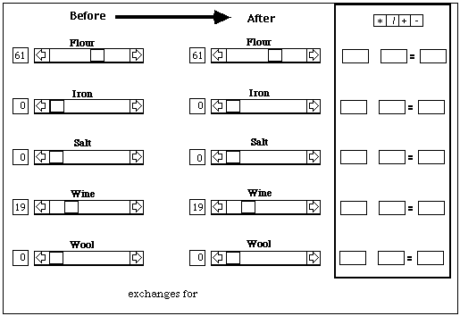
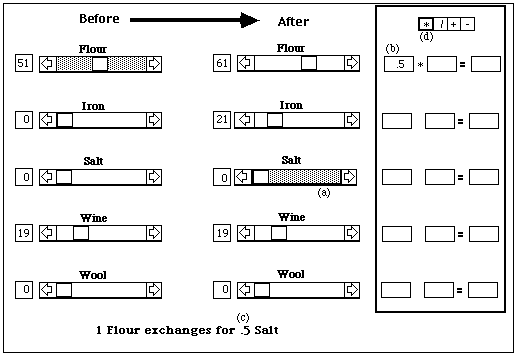
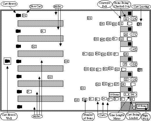
  • The figure shows the situation at the beginning of the player's move. He has 61 units of flour, 19 units of wine, and no iron, salt, or wool. Since he has not yet specified any trades, quantities after are the same as quantities before. Since he has not selected any good to trade, all of the scroll bars are blank, indicating that they are not active. Since he has not yet made any use of the calculator at the right of the screen, all of its boxes are blank.


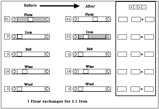
    The next figure shows the situation after the player has tentatively decided to trade 10 units of flour for iron. He selected flour by clicking on its scroll bar in the Before column, iron by clicking on its scroll bar in the After column. The bottom of the screen shows him the rate at which flour exchanges for iron. Moving the scroll box for flour 10 units left moved the scroll box for iron 21 units right, since 1 unit of flour exchanges for 2.1 units of iron.


  •  


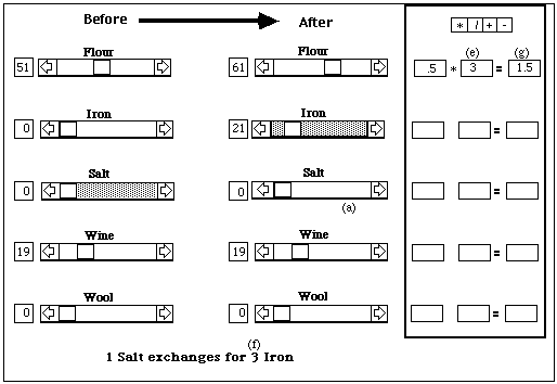
  • The next figure shows how the calculator is used. Suppose the player wishes to compare two alternative ways of getting iron from flour &endash;direct trade vs trading flour for salt and then salt for iron. He knows that the former method gives him 2.1 units of iron for each unit of flour. To find the return from the latter method, he first clicks on salt in the After column (a), then clicks on one of the left-hand boxes in the calculator region (b), then clicks on the number shown at the bottom of the screen as the rate at which flour exchanges for salt (.5) (c). Next he clicks the * icon at the top of the calculator box (d), to specify that he wants to multiply the two numbers that will be in the left and middle boxes of one of the rows of boxes on the calculator region; this is the point in the process illustrated in the figure below.


  •  


  • Next the student selects salt in the Before column and iron in the After column; the screen now shows at the bottom that 1 unit of salt exchanges for 3 units of iron. He clicks on the middle box of the calculator region (e). He next clicks on the number 3 at the bottom of the screen (f), which then appears in the middle box; the product of .5 and 3 appears in the right hand box of the calculator region (g), as shown in the next figure. The student observes that he is better off getting iron by the direct trade. If he is clever, he realizes that this means he can profit by trading flour for iron, iron for salt, and salt for flour.


    Further Notes


    In showing the interface, I have assumed a single set of five goods. It might be desirable to use those goods for what I have called version 2 of the program, and a set of currencies for version 1, thus distinguishing the two in the eyes of the students. It seems intuitively more plausible that one arbitrageur would influence the price of flour in a village than the price of marks on the international currency market.


  •  


  • Note that the exchange rate shown at the bottom of the screen (as in "1 Salt exchanges for 3 Iron") is a constant in version 1 of the program but varies slightly as the player varies the amount he plans to trade in version 2; in either case it shows the ratio of number of units received to number given up if he makes the trade currently selected.


    It might be desirable to allow the student to display marginal revenue as well as price, since in version 2 they are not equal. Marginal revenue would be the increase in the number of units (say of iron) he gets as a result of giving up one more unit of (say) salt.


    It would also be desirable to allow a student who has set up his trades for the turn and decides he does not like them to go back to the situation at the beginning of the turn; that might be a menu selection with a keyboard equivalent.


    Strategies


    The game, in all of its versions, permits three different strategies for winning. One strategy is pure speculation; the player acquires stocks of good that he expects to go up in relative price and gets rid of stocks of goods that he expects to go down. This strategy might work if the player either is lucky or takes advantage of the predictable element in price movements&endash;their tendency to move towards consistency.


    The second strategy is pure arbitrage. To engage in pure arbitrage, the player first acquires stocks of at least three different goods. When the prices for those three goods are inconsistent he can, in a single turn, make simultaneous transactions on all three markets (ij, jk, ki) whose combined effect is to leave him with unambiguously more than he started with.


    The third strategy is a mix of the two. A player with a stock of good i observes that the prices on the ijk market are inconsistent&endash;he could gain by trading i for j, j for k, and k for i. He trades units of i for j this turn. His plan is to trade j for k next turn and k for i the turn after. The problem with the plan is that the inconsistency will, on average, be decreasing over time, and in addition will have some random change in it.


    Economics Note


    I have implicitly assumed that, arbitrage aside, there is no connection between, say, the wool-steel market and the flour-steel market. An individual consumer/producer is interested in only two goods. Someone who trades wool for steel has nothing else to trade for steel and wants nothing else that wool can be traded for, so the price on that market is unaffected by prices on any of the other nine markets. This is obviously unrealistic, but greatly simplifies the modelling. One could construct a fancier set of equations to eliminate this assumption, but I doubt it is worth the trouble.


    Alternative Interface: Four Currencies


    In this version, everything is done by dragging piles of bills around the screen. When a pile is dropped in a different region, it converts and goes grey (assuming only one transaction is permitted per turn). Until the turn is over it can be dragged back. At the end of the turn, all dollars are combined into one pile, etc.


    In any version, you can click on a stack, control z takes it back one step, shift control z takes it to where it started the turn. Shift click to select a bunch of stacks and do the same.


    Alternative Games (1992 version)


    1. One player, any number of trades. Each bill can only make one loop. There is a time limit within which to find the best trade. Everything ends up back as dollars.


    2. One player, one trade per bill per turn. At the end of each turn, exchange rates are recalculated.


    3. As in 2, but trades shift exchange rates towards consistency. Price shifts continuously as you trade; trades cannot be undone (save at new price).


    4. As in 3, but relative prices are continually shifting (real time)


    5. Multiple players, either consecutive (one machine) or simultaneous (network version). In the simple consecutive one, trades shift prices at the end of a player's turn, some randomness then added between turns. Alternatively, like 4. On the network, prices move continuously, trades cannot be undone.
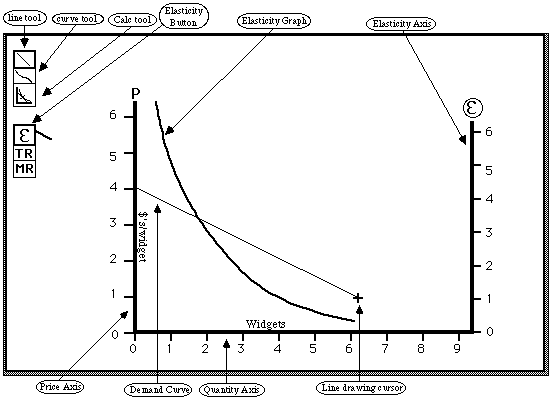


    Elasticity, TR, MR


    Student draws a demand curve. Program shows elasticity at any point, shows TR and MR at request.


    The Lesson


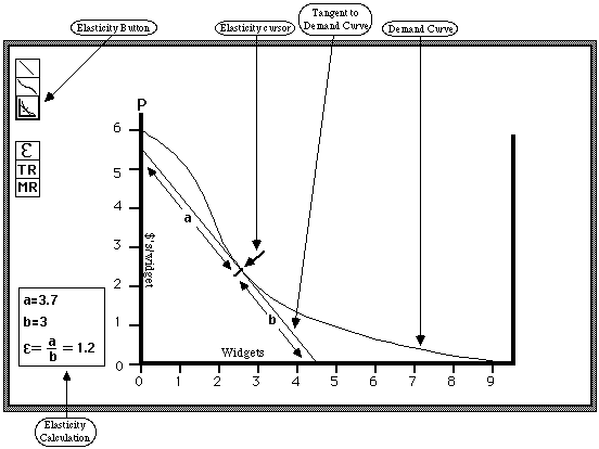
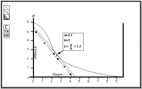
    One of the things students learn about in Principles and Intermediate Microeconomics courses is elasticity. The elasticity of a demand curve is defined as minus the limit for small changes of the percentage change in quantity divided by the corresponding percentage change in price.


    The purpose of this program is to give the student an intuitive feel for what elasticity is. It does so by letting him draw a demand curve and showing him the elasticity of that curve as a function of quantity. Ideally, the student should be able to modify the curve and watch how the elasticity is affected.


    One of the reasons elasticity is important is that it is closely related to total revenue and marginal revenue. If total revenue is at a maximum then demand elasticity is one and marginal revenue zero. The program will also let the student view the total revenue and marginal revenue curves implied by his demand curve.


    There is a simple geometric trick for calculating elasticity, discussed in my textbook and some others. The program will allow the student to see that the results of calculating it in that way are the same as those shown by the program.


    In summary, the lesson of this program is a more intuitive understanding of the relation among a demand curve, its elasticity, and the total and marginal revenue functions it implies.


    Program and Interface


    I will describe two versions of the program, of which the second is better and harder to program. In the first version a demand curve is drawn but cannot be modified; if the student wants to look at a slightly different demand curve he starts over and draws it from scratch. In the second version the student can adjust the curve after it is drawn and watch the changes inelasticity, TR and MR.


    Version 1


    The student is presented with a set of axes. The vertical axis shows price; the horizontal shows quantity. He selects either a straight line or a curve tool from a tool palette on screen and uses it to draw a demand curve. The straight line tool works like the line drawing tool in MacDraw or MacPaint. The curve drawing tool has a built-in smoothing feature to compensate for the usual shakiness of a mouse-drawn curve; the curve, instead of exactly following the cursor, grows towards the cursor, with the speed proportional to the distance between the cursor and the end of the curve.


  •  


  • Either before or after drawing the demand curve, the student can use on-screen buttons to choose which other curves are to be shown; the alternatives are elasticity, total revenue, and marginal revenue. If another curve (or curves) is selected before the demand curve is drawn, the student sees that curve(s) appear as he draws the demand curve. After drawing the demand curve, the student can select the Calc tool. With this tool selected, he can click anywhere on the demand curve and see how elasticity is calculated at that point.


    The figure above shows the screen as a straight line demand curve is being drawn. The line tool is highlighted; the cursor is in the shape of a cross. The student has also selected elasticity, with the result that elasticity is also being drawn in. Note that there is a separate elasticity axis with different units, to remind the student that the vertical axes of the two graphs represent different things.


    This suggests a problem. What if two different things are selected, such as elasticity and TR? There is only one right hand axis. Which variable does it represent?


    The program lets the student decide. e in the figure above is located inside a circle. That circle is in fact a button. If two or more graphs are selected, clicking on the button cycles the right hand axis through its alternative forms, changing the label, the numbers, and the units. On the figure above the right hand axis has no units, since elasticity is a pure number, but there would be units for TR or MR.


    If several different things are being drawn at once, the figure is likely to become confusing. To reduce that confusion the different variables should be represented by different kinds of lines. On the figure above, a thick line is used for elasticity and a thin line for demand. Dashed lines, greyed lines, or colored lines on appropriate hardware would provide the same effect for more alternatives. To make it clear which line applies to which alternative, the line should be shown next to the palette choice. The figure below shows how that would look with elasticity and total revenue both selected. Total revenue is represented by a dashed line.


    Version 2


    This works just like version 1, with one major change. After a demand curve has been drawn, the student can select an adjustment tool. This tool works like "reshape" in Macdraw. Black boxes appear at intervals along the curve. The cursor can be used to move these boxes; demand is a smoothed curve approximating the series of boxes. Thus moving the boxes allows the student to change the shape of the curve. As he does so, whichever other curves he has selected for display (elasticity, TR, MR) change as well.


  •  

  •  
    The Calc Tool


    The figure above shows how the calc tool is used. A demand curve has been drawn, using the curve drawing tool. The student has then selected the calc tool and clicked on one point of the demand curve. The screen shows how the elasticity at that point is calculated as the ratio of the two segments of the tangent to the demand curve at that point.


    Note that since none of the graphs (elasticity, TR, MR) is selected, the right axis has no labels. The elasticity calculation is shown in a box to the left of the drawing area. The next figure shows an alternative way in which it might be displayed.


    One problem which might arise in using the calc tool is insufficient screen space; the tangent might intersect either the vertical or the horizontal axis (or both) off screen. The elegant solution would be for the program to automatically shrink the demand curve, relabelling the axes accordingly, so that the figure would fit.


  •  


  •  
    Mathematics


    The demand curve can be represented by a function Q(P), showing quantity as a function of price. Elasticity is then:


    Total revenue is simply price times quantity:


    TR=PQ(P)


    Marginal revenue is the derivative of total revenue with regard to quantity.


    Supermarket Seen From Above


    Student controls the parameters, watches the equilibrium.


    Lesson


    Economics frequently deals with equilibria maintained by negative feedback. A simple example of such an equilibrium is the system of checkout lines at a supermarket. Individual shoppers try to go to the shortest line, and by doing so tend to keep the length of the lines approximately equal. The situation can be used to illustrate a variety of economic concepts, such as search costs, corner solutions, rationality in the presence of imperfect information, etc. The example is discussed at some length in my book Price Theory: An Intermediate Text; a copy can be made available to programmers if necessary.


    The purpose of this program is to give the student a feel for the logic of such equilibria by letting him watch a model of a set of supermarket lines. The student can alter various features of the situation and observe the effect. At the simplest level the lesson is an understanding of how and why negative feedback makes all lines equal and how, in a corner solution, it fails to do so. At a higher level, the model shows how rational search, whether for the shortest line or for other information relevant to the correct choice, ends up, in equilibrium, generating equally attractive outcomes for those who do and do not choose to search.


    Program and Interface


    The figure below shows the program's display window&endash;a view of a supermarket from above. Individual shoppers are represented by their shopping carts; the number of items that each shopper has is represented by a number in the cart.


    The carts originate in cart sources, shown as solid black carts. In the figure, the cart source in the top aisle has just generated a cart with 31 items in it. A cart source represents the point at which a shopper, having found the last item he wants, starts towards the front of the store to check out.


    Each turn each cart source has a probability pc of generating a cart. The figure shows one cart source in each aisle. That implies that, on average, the same number of shoppers are appearing in each aisle. The student can use the mouse to move the cart sources; if, for instance, he put all of them in the first aisle, then all shoppers would finish shopping there. The student can get additional cart sources from the cart source well, or eliminate cart sources by dumping them into the cart source well.


  •  


  • Changing the number of cart sources does not change the total number of carts appearing each turn. That total, <Nc>, is determined by the demand curve and the length of the lines, as explained below. As the total number of sources changes, pc changes in the opposite direction to keep their product, <Nc>, constant.


    After a cart appears it moves forward, joins the end of a line, moves towards checkout, unloads its items, is reloaded with bags full of checked out groceries, moves farther forward, and vanishes as the shopper exits the store. The length of time required to check out a given shopper is equal to the number of items he has plus three; two shoppers with three items each take as long as one with nine. A line length meter at each checkout station shows the student (but not the shopper) how long it will take the last shopper in that line to get through; the number on the meter is the number of items in the line (including items unloaded onto the conveyor belt but not yet checked through) plus three times the number of carts in the line (not counting the one that has already been unloaded onto the conveyor belt). The function of the meter is to let the student see how waiting time varies from line to line.


    Demand


    The total number of shoppers entering the store each hour depends on the demand curve for groceries and the cost. The demand curve can be viewed and altered by the student. It appears in its own window, accessible by a menu choice and superimposed on the supermarket window, as shown below. Like any window, it can be moved; thus the student can, if he wishes, put the demand window over some part of the display window and watch both functioning at once. The figure below shows the display window with both the demand window and the search window (explained below) on top of it.


  •  


  • The cost of groceries is the sum of the price and the waiting cost. The waiting cost is simply the average over all shoppers of the time it takes to get through the line&endash;including any search costs (explained below).


    The student can change the demand curve with the mouse by grabbing one end or the other and moving it. He can change the price by grabbing the price line and moving it up or down. The waiting cost is being determined within the program, so he cannot directly control it.


    Search Strategies


    So far I have not described how the individual shopper decides which line to put his cart in. The program permits the student to choose any of a range of search strategies, as follows.


    I. No search: The cart emerges from its aisle in between two lines, and goes to whichever of the two has fewer carts in it.


    II. Item Counting: Some fraction of the carts FI belong to shoppers who base their choice not only on the length of the line but on the number of items in the carts near the end. They look at the last NII carts in each of the two lines, where NII is a positive integer chosen by the student, and count the number of items in each. They then estimate the time length of the lines, assuming that the remaining carts each have the average number <I> of items in them, where <I> is the average of the distribution of number of items generated by the cart sources. Having estimated the time length, such shoppers go to the shorter line.


    III. Line Search: Some fraction of the carts FL belong to shoppers who check more than the two nearest lines; NIII is the number of lines each such shopper checks. Such a shopper moves his cart to a point behind the shorter of the two lines. From there he can see a third line. If NIII=3 he then goes to the shortest of the three lines, unless moving to it would take long enough to more than wipe out the difference in time between it and the line he is now behind. If NIII>3 he moves on and checks another line, and continues until he has seen NIII lines. He then goes to the shortest line, again including in length the time it will take him to get from where he is to the line.


    IV. Strategies III and IV can be combined; the shopper can check several lines, counting items in each. It would probably be desirable to have only one search strategy in use at a time, however; an individual shopper either uses that strategy or he engages in no search, as described under I.


    Search strategies can be set from a menu and observed in a search window. The student chooses whether to have some shoppers following I, II, or III, how many (what fraction), and in what form; in other words, he picks NII or NIII and FL. The window then shows both what strategy is selected and its outcome.


    The outcome is shown as average time to get out of the supermarket for searching and non-searching customers. The average is taken over the last ten customers of each sort to exit the store&endash;or fewer if fewer than ten have exited since the last change in search strategy. Time for searching customers is shown as the sum of search time and time in line. The program has built into it the cost in time to count items and the cost in time to move from one line to another. The figure below shows the search window; like the demand window, it can be open and visible while the display window is visible and functioning. The figure above shows a search window open; the details of what is displayed correspond to the Rational Search option described below.


    Carts which are following a search strategy should be distinguished in some way. One possibility would be to have the cart blink while it searching. Another possibility would be to put the number of items in that cart in boldface.


    Express Lanes


    The student can, if he wishes, set one or more lanes as express lanes and set the maximum number of items which a customer is allowed to take through an express lane. A customer with more than that number of items ignores the express lane. If he is between it and a normal lane and he is following the no search strategy he goes to the regular lane. A shopper permitted to go through the express lane estimates its time length assuming that the carts in line each contain <Ie> items, where <Ie> is the average over carts containing no more than the permitted number of items. He then goes to the lane which he estimates to have the shorter time cost.


    Express lanes are set by taking an express lane sign from the sign well at the lower right hand corner of the display window (shown on the previous two figures) and putting it next to the appropriate lane. Before taking the sign from the well, the number of items is set by clicking on the up arrow next to the well to scroll the number up or the down arrow to scroll it down.


    Rational Search


    So far, the search strategies of the shopper have been chosen by the student. We would expect, however, that if searching several lines before choosing one is on average a successful strategy&endash;if the savings in time spent in line is greater than the cost in time spent searching&endash;then the number of searchers will increase. Similarly, we would expect that if, on average, searching one more line results in a reduction in search time plus waiting time, the number of lines searched will increase. So if we allow shoppers to rationally choose strategies the parameters of search&endash;the fraction of shoppers searching and the amount of search in lines checked or carts examined for number of items&endash;become endogenous.


    The student can select or deselect rational search on a menu. With rational search selected, the student can still choose the form of search (item counting or line search or both) and the parameters. But the parameters chosen are now only starting values. If, on average, search pays, then the fraction of shoppers searching increases; if search costs more than it is worth, the fraction decreases. If NIII, the number of lines being searched, is initially set to 4, then most searchers search r lines but a few, randomly chosen, search 3 or 5. If either variant produces a better outcome than 4, the number choosing that variant increases. Once most searchers are searching (say) 5 lines, all of those searching 3 switch to 4 and a few start searching 6. A similar mechanism applies to number of carts checked in strategy II.


    With Rational Search enabled, the search window shows all of the strategies being followed, what fraction of shoppers follow each, and the current payoff to each. Where possible, the information should be shown in graphic form. The figure shows one way in which this could be done; fractions of shoppers are shown as a horizontal bar graph, payoff is a vertical bar above each part of the horizontal bar. In the case shown, the search strategy is III and the depth of search of measured by number of lines checked.


    Supermarket as a Game


    So far, the program is a simulation intended to help a student understand economic concepts by letting him watch them in action. It could be designed to also function as a game, in which the student tries to maximize the supermarket's profits. This would require only minor modifications to the program.


    The first modification would be to have the program choose (randomly each play) an average cost per item, shown as a horizontal line on the demand graph. The second would be to compute current profit per hour and a running total of profit for the day and report them&endash;again probably in the demand window. I will assume in this discussion that one play of the game corresponds to operating the supermarket for one day.


    If the student represents the supermarket manager he cannot be free to control the demand curve. When the program is played as a game demand should either be constant at a level set randomly each play (simple version) or vary in a largely predictable fashion during the course of a day (hard version). In either case, the scoring system should compensate for random elements, so that the score measures how well the student did relative to the highest profit that could be produced by perfect play. Time of day should be shown on a clock somewhere on the display screen.


    The student as supermarket manager can set price. The game will be more interesting although less realistic if he can vary price during the day, both in order to experiment with the effect of different prices and to respond to changes in demand. The student should be able to play the game with different search options enabled, but that should represent a choice of what game to play rather than a strategy for winning, since the supermarket manager does not control the behavior of the customers. A particularly interesting version would be one with Rational Search enabled.


    While the manager does not control the strategies of the customers, he may be able to affect their cost. One of the choices open to the student should be to install, at some cost, mirrors in the ceiling above the checkout lanes, making it much easier for shoppers to see how many items the carts in each lane have and how many carts are in each line. The program would reflect this by expanding the range of free search from the two adjacent lines to also include the two lines adjacent to them, and lowering the cost of counting items. It would be up to the student to figure out whether this increases his profits.


    Present Value Visual Calculator


    The student calculates the present value of a sum of future payments, using a visual calculator on which a values is represented as the height of a line.


    Lesson


    The purpose of this program is to give the student some intuitive feel for the workings of compound interest, both backwards (present value) and forwards (future value). It does so by letting him calculate the present or future value of a sum of payments by picking a payment size, moving the location of the payment in time, and seeing as he does so how the present (or future) value changes. Stacking such payments corresponds to adding them.


    The Program


    (Version 1, present value)


    The interface shows a left-hand vertical axis, representing value discounted to time 0, a right hand vertical axis, representing value at time T, and a horizontal axis representing time, with T at its right end. If a dollar at T has a present value of fifty cents (this depends, of course, on the interest rate and T), then the right hand axis is half as tall as the left-hand axis, and all measurements are half as large.


    The student chooses a value by clicking at the appropriate height on the left hand axis. A vertical bar appears with that height, representing a payment of $D at time 0. D is written (vertically) on the bar. The student can use the mouse to slide the bar right along the time axis. As he does so, it shrinks, so that its actual height when it is moved to time t equals the present value at time 0 of $D at time t. As he moves it, the bar casts a "shadow" of its (shrunken) height on the left-hand axis, so you can see numerically what the present value is.


    Suppose the student wants to find the present value of a sum of payments. He chooses the first payment as described above, and moves it to its appropriate time location. He then chooses a second payment; the first bar goes grey, its shadowing lines disappear, but its (grey) shadow remains on the left-hand axis. When the second payment is at the appropriate point, the student clicks a + button, and the shadow of the first payment is shifted vertically so that its bottom is at the top of the shadow of the first payment and its top represents the sum of the present values. The process can be continued for additional payments. At any point, the student can click on any payment and its shadow and shadowing lines appear.


    At any point in the process, the student can change the interest rate and see the effect on the calculation.


    Screen after choosing $10,000 payment, moving it to year 6


    Screen after selecting second ($14,000 in year 4) payment


    Screen after adding two present values


    (Version 2, future value--the power of compound interest)


    This is the same as version 1, except that choosing, shadowing, adding, etc. is done on the right -hand axis, so that the student is calculating the sum at time T of interest and principal from a series of earlier payments.


    (Version 3, inflation)


    In this version, the student gets to set both the real interest rate and the inflation rate, use real or nominal magnitudes, and change among them. Among other things, he should be able to see the same series of payments as nominal, present value, or real.


    Cleaning Out Cobwebs: Speculation vs the Hog/Corn cycle


    This program does two things--it shows how the cobweb theorem works and why it doesn't work. It does the first by letting the student draw the relevant curves, pick a starting point, and watch the cobweb draw itself on the demand supply diagram, while quantities and prices are graphed against time on another diagram. It does the first by letting the student add speculators to the system, giving each a starting sum and buy and sell points. The program than shows the smoothing effect of speculation in either or both markets. A simpler version may show the same thing with one good, where producers decide on output in terms of last period's price.


    The Program


    (Version 1--one good)


    The student draws straight-line supply and demand curves for one good in one window, then clicks somewhere on one curve to start things going. If it is on the supply curve, price adjusts to the price for which that quantity will sell (i.e. move vertically to demand curve). Quantity then adjusts to the quantity produced at that price (i.e. move horizontally to supply curve). Continue, until you converge to the intersection of the two curves or go off the graph.


    Meanwhile, in another window, the program graphs price and quantity against time, assuming that each step takes one year.


    The student may now introduce a speculator. The speculator buys goods at one time and holds them to sell at another; initially his storage cost is zero. The speculator starts with a fixed amount of money, a price at which he buys, a higher price at which he sells. The student re-runs things (i.e. hits a "start over" button, and watches how the sequence is changed by the presence of the speculator. The second window now also graphs the speculator’s wealth, defined as his cash holding plus the market value of the goods he holds. The student may increase the number of speculators, adjust speculator’s wealth and buying strategy, etc., and watch the effect.


    A possible further addition would be a "rational expectations" speculation option. Instead of having fixed buy and sell points, the speculator follows whatever strategy maximizes profits, given that he knows the logic of what is happening.


    (Version 2)


    This is essentially the same, except that there are two goods, corresponding to the classical analysis of the Hog/Corn cycle. The student draws initial demand and supply curves for both goods, in two different windows. The program then moves the demand curve for corn according to what is happening in the hog market, and the supply curve for hogs according to what is happening in the corn market, according to the standard analysis.


    Milton Keynes.


    The student combines the roles of Secretary of the Treasury and Chairman of the Fed. He gets to control the supply of high powered money and suggest a total level of taxation (and possibly of expenditure). Before choosing his variables, he is told what the administration expects expenditure to be. After choosing his variables, he observes the resulting levels of expenditure, inflation, real GNP, interest rates, unemployment, and satisfaction. The game continues either for a fixed number of years or until the player does so badly that he is fired.


    What makes the game interesting is that the player does not know the system of equations underlying the computer’s response to the player’s actions. The system may be simple Keynesian or simple Monetarist. In addition, Congress, in setting actual levels of taxation and expenditure, may be trying to do good or controlled by Public Choice considerations.


    One might have a two player version, in which one person controls money and one proposes a budget, with different but correlated maximands for the two people.


    The Program


    The player starts by filling out an employment form (Position: Secretary of the Treasury); information from that form is used in generating news stories later on. Then play starts. The computer randomly determines the structure of the economy, subject to the difficulty level that the player has chosen. Players also have the option of playing with a known structure of the economy, as a "practice game."


    In all versions, government expenditure produces some public goods but reduces private production via disincentives. The net result is that, macro effects aside, there is some optimal level of Federal expenditure; lower levels result in lower GNP (inadequate public goods); higher levels result in lower GNP (wasteful government spending). Both effects may be reflected in Newspaper articles. What the optimal level is will vary from play to play, between a low of 3% (U.S. pre WWI) and a high of 35%.


    At any time, the player can click on a Newspaper Icon, opening a window showing a current newspaper. There will be several different papers, with different slants. Some of the contents will be noise, some useful information, such as hints at the public choice forces driving expenditure, stories suggesting wasteful government spending or inadequate production of public goods, or a final story announcing the sacking of the Secretary of the Treasury.


    In the monetarist version, the price level is proportional to the quantity of high powered money divided by the GNP; the proportionality constant may be dependant on the nominal interest rate. GNP is driven by real forces. Unemployment is low when the money supply increases more than expected, high when it increases less than expected. Low unemployment increases satisfaction in the short run but lowers it in the long, as workers discover they are getting less than they thought. Real interest rates are an increasing function of the deficit (unless we want to build in the Ricardo Theorem).


    In the Keynesian version, the economy is sometimes but not always in underemployment equilibrium. If it is, increases in high powered money have no effect; if it is not, they cause inflation. Taxation and expenditure have the usual Keynesian effects.


    If Public Choice applies, expenditure tends to increase to absorb surpluses. We also might want to put in a political business cycle--Fed and treasury policy deviate from what the player wants in the direction of short-term increases in satisfaction in election years.


    The player is scored by one of several measures; which is used might be chosen by the player at the start of play or by the computers. Some possibilities are average real GNP (possibly present value), real GNP at end of game, average of the sum of unemployment and inflation rates, and average satisfaction.


    Economics Programs


    Contents

    We plan to produce between twenty and thirty programs, designed to teach economic concepts at the elementary and intermediate level. None will be programmed instruction in the conventional sense--that is to say, none will consist of simply showing a series of words and pictures on a computer screen instead of a sheet of paper. All will be interactive, some in the form of games. A much more detailed description of the programs is available.

    Licensing Terms

    The programs will be available to be licensed to textbook publishers on a non-exclusive basis. We will charge $3000 per book for customizing them to fit a particular textbook. Customizing will consist of working with the publisher or author to decide which programs (in some cases, which parts of which programs) are suitable for that particular book. In addition, we will provide the author with the tools necessary to edit the on-disk help information, in order that he can add references to specific parts of his book, maintain consistent terminology, and so on.

    In addition to the customization charge, we will charge a royalty of $.20/copy for every copy of the book sold. In exchange for this payment, the publisher gets the right to make the customized version of the programs available to any or all students using the book. This could be done by enclosing a disk with every copy, selling disks separately, or providing disks free to adopting professors, with permission to make copies for their students. However it is done, the royalty is charged on the book not the disk, since one disk sold or given away may result in many students having copies of the programs.


    The programs will initially be produced on the Apple Macintosh and then on some version of the IBM PC; the PC version will require some form of graphics, and will therefore not run on all machines. Publishers that wish to distribute the Macintosh version only, prior to the availability of the PC version, will be charged a royalty of only $.10/copy for doing so.


    Schedule


    We currently hope to have the programs available by Christmas of 1990. Prototypes of a considerable number should be available to be shown sometime in the spring of 1990. The initial suite of programs will be in microeconomics; we hope later to produce additional programs for macro textbooks.


    Revisions


    Minor revisions and bug fixes will be provided free to publishers who have licensed the programs.


    More program ideas


    Programs for the math review that often goes with econ. Curvedraw Mk II. Also an analytic geometry program. Type x, point moves out x axis. Type y, goes up to (x,y) location. click on any point, get coordinates. Maybe type in (or click on) function, get it graphed.


    Arcade version. Target on screen. Type in coordinates. Shoot. Against time. Or run backwards--program gives coordinates, you use mouse to locate.


    Monte-Carlo program. Demonstrate the central limit theorem. Possibly demonstrate spurious cycles via random numbers (see below).


    Regression program. Pick a real relation y=a+bx. Plot points with errors. As each point is added, calculate regression line, show it plus zone of lines corresponding to error in estimates of a and b.


    Going from a utility function to an indifference curve. Student specifies utility function (or chooses from a set of alternatives). Picks values of x and y, observes utility. Picks new value of one, adjusts the other until "boing" same utility. New point plotted. Repeat. In the process, generate MRS along the curve. Draw B line, generate MRT. Observe intersection, especially at tangent for tangent.


    Cycle, cycle, who’s got the Cycle: two "business cycles," one generated by coin flips or the equivalent, the other a sign curve plus error, both with points limited to the same grid (± integral number of coin flips). Sign curve has random period. Student clicks as soon as he is sure which is the cycle. (or Bi-Cycle?) [A preliminary version of this now exists as Grglflx]


    Hotelling theorem program. Student picks initial amount of depletable resource, interest rate, probability of expropriation. Program graphs price and quantity over time. In a fancier version, student can pick cost curve for production, and perhaps let it change over time.


    Limits to growth done right. A simple interacting system, shown with and without prices as negative feedbacks. Program graphs out path over time.