Chapter 13
Chapter 13
. . . And Chance
I returned and saw under the sun, that the race is not to the swift, nor the battle to the strong, neither bread to the wise, nor yet riches to men of understanding, nor yet favour to men of skill; but time and chance happeneth to them all.
-- Ecclesiastes 9.11
PART 1 - SUNK COSTS
So far, I have introduced time into the economy, but not uncertainty; everything always comes out as expected. The real world is not so simple. One of the consequences of uncertainty is the possibility of mistakes; another is the problem of what to do about them.
You see an advertisement for a shirt sale at a store 20 miles from your home. You were planning to buy some new shirts, and the prices are substantially lower than in your local clothing store; you decide the savings are enough to make it worth the trip. When you arrive, you discover that none of the shirts on sale are your size; the shirts that are your size cost only slightly less than in your local store. What should you do?
You should buy the shirts. The cost of driving to the store is a sunk cost--once incurred, it cannot be recovered. If you had known the prices before you left home, you would have concluded that it was not worth making the trip--but now that you have made it, you must pay for it whether or not you buy the shirts. Sunk costs are sunk costs.
There are two opposite mistakes one may make with regard to sunk costs. The first is to treat them as if they were not sunk--to refuse to buy the shirts because their price is not low enough to justify the trip even though the trip has already been made. The second is to buy the shirts even when they are more expensive than in your local store, on the theory that you might as well get something for your trip. The something you are getting in this case is less than nothing. This is known as throwing good money after bad.
When, as a very small child, I quarrelled with my sister and then locked myself in my room, my father would come to the door and say, "Making a mistake and not admitting it is only hurting yourself twice." When I got a little older, he changed it to "Sunk costs are sunk costs."
In discussing firms' cost curves, one should distinguish between fixed costs and sunk costs--while the same costs are often both fixed and sunk, they need not always be. Fixed costs are costs you must pay in order to produce anything--the limit of total cost as a function of quantity when quantity approaches zero. One could imagine a case where such costs were fixed but not sunk, either because the necessary equipment could be resold at its purchase price or because the equipment was rented and the rental could be terminated any time the firm decided to stop producing.
The significance of sunk costs is that a firm will continue to produce even when revenue does not cover total cost, provided that it does cover nonsunk costs (called recoverable costs), since nonsunk costs are all the firm can save by closing down. All costs, ultimately, are opportunity costs--the cost of doing one thing is not being able to do something else. Once a factory is built, the cost of continuing to run it does not include what was spent building it, since whatever you do you will not get that back. It does include the cost of not selling it to someone else--which may be more or less than the cost of building it, depending on whether the value of such factories has gone up or down since it was built.
In deriving the supply curve for a competitive industry with open entry in Chapter 9, we saw that firms would always produce at the minimum of average cost, where it crossed marginal cost. The reason was that if, at the quantity for which marginal cost equaled price (where profit is maximized for a price taker), price were above average cost, economic profit would be positive; it would pay other firms to enter the industry. They would do so until price was driven down to the point where it equaled both MC and AC, which occurs where they cross at the minimum of AC.
Does the relevant average cost include sunk costs? That depends on whether we are approaching the equilibrium from above or below and on how long a time we consider. If prices start out above the equilibrium price, firms will only enter the industry as long as the price is above average cost including sunk cost--costs are not sunk until they are incurred, and the new firm starts out with the option of not incurring them. The equilibrium will be reached when price equals average total cost.
If we approach the equilibrium from below--if there are too many firms (perhaps because demand has recently fallen) and price is insufficient to cover even the average of recoverable costs--firms will leave the market. They will continue to do so until price gets up to average recoverable cost.
If the assets bought with the sunk costs (factories, say) wear out over time, then the number of factories will gradually decline and the price will gradually rise. Until it reaches average total cost, nobody will build any new factories. Eventually price will be equal to average total cost, just as it was when we reached the equilibrium from above, but it may take much longer to get there; it usually takes longer to wear out a factory than to build one.
In the next two sections, I will work through the logic of such situations in some detail while trying to show how it is related to the logic of a different sort of situation that was briefly discussed several chapters ago.
In analyzing the industry supply curve in Chapter 9, I assumed an unlimited number of potential firms, all with the same cost curve; if existing firms make a profit, new firms come into existence until the profit is competed down to zero.
One objection to this that I discussed is that firms are not all identical. Some power companies own special pieces of real estate--Niagara Falls, for example--not available to their competitors. Some corporations are run by superb managers or possess the services of an inventive genius such as Browning or Kloss. Surely such fortunate firms can, as a result, produce their output at a lower cost than others--and can therefore make profits at a price at which it does not pay less fortunate firms to enter the industry.
But although firms that have, in this sense, low cost curves appear to make positive profits when less fortunate firms just barely cover their costs, that is an illusion. One should include in cost the cost of using the special assets (location, administrator, inventor, or whatever) that give that firm its advantage. The value of those assets is what the firm could sell them for or, in the case of human assets, what a competitor would pay to hire them away. One of the firm's (opportunity) costs of operating is not selling out, and one of the costs to an inventor of running his own firm is not working for someone else. If the possession of those special assets gives the firm an additional net revenue of, say, $100,000/year (forever--or almost), then the market value of those assets is the present value of that income stream. The interest on that present value is then the same $100,000/year. Since giving up that interest is one of the costs to the firm of staying in business, the firm should subtract it from revenue in calculating its economic profit.
Suppose, for example, that the firm is making an extra $100,000/year as a result of owning its special asset and that the interest rate is 10 percent. The present value of a permanent income stream of $100,000/year is $1,000,000, and the interest on $1,000,000 is $100,000. By using the asset this year, the firm gives up the opportunity to sell it and collect interest on the money it would get for it. We should include $100,000/year as an additional cost--forgone interest. Doing so reduces the profit of the firm to zero--the same as the profit of an ordinary firm. In one sense, this argument is circular; in another sense, it is not.
The same argument applies in the opposite direction to firms whose revenues fail to cover their sunk costs (firms whose revenues fail to cover their recoverable costs go out of business). Suppose a widget factory costs $1,000,000 to build and lasts forever; further suppose the interest rate is 10 percent, so that the factory must generate net revenue of $100,000/year to be worth building. At the time the factory is built, the price of widgets is $1.10/widget. The factory can produce 100,000 widgets per year at a cost (not including the cost of building the factory) of $0.10/widget, so it is making $100,000/year--just enough to justify the cost of building it. Further suppose that the factory can be used for nothing but building widgets; its scrap value is zero.
The invention of the fimbriated gidget drastically reduces the demand for widgets. Widget prices fall from $1.10 to $0.20. At a price of $0.20, the firm is netting only $10,000/year on its $1,000,000 investment. So are all the other (identical) firms. Are they covering costs?
The factory is a sunk cost from the standpoint of the industry, but any individual firm can receive its value by selling it to another firm. How much will it sell for? Since it generates an income of $10,000/year and since at an interest rate of 10 percent an investment of $100,000 can generate the same income, the factory will sell for $100,000. So the cost of not selling it is $100,000--and the annual cost of not selling it is $10,000, the interest forgone. Ten thousand dollars is the firm's revenue net of costs before subtracting the cost of the factory, so net revenue after subtracting the cost of the factory--economic profit--is zero.
Again the argument is circular but not empty, since it tells us, among other things, what determines the price of a factory in a declining industry. In the case I have just described, the firm loses $900,000 the day the price of widgets drops, since that is the decrease in the value of its factory. Thereafter it just covers costs, as usual.
The assumptions used in this example, although useful for illustrating the particular argument, are not quite consistent with rational behavior. In the market equilibrium before the price drop, economic profit was zero. That is an appropriate assumption for the certain world of Chapters 1-12, but not for the uncertain world we are now discussing. If there is some possibility of prices falling, then firms will bear sunk costs only if the average return justifies the investment. Prices must be high enough that the profit if they do not fall balances the loss if they do. The zero-profit condition continues to apply, but only in an average sense--if the firms are lucky, they make money; if they are unlucky, they lose it. On average they break even. This point will be discussed at greater length later in the chapter.
You may find it helpful to work through another example. Consider ships. Suppose that the total cost of building a ship is $10,000,000. For simplicity we assume that operating costs and the interest rate are both zero. Each ship lasts twenty years and can transport 10,000 tons of cargo each year from port A to port B. We assume, again for simplicity, that the ships all come back from B to A empty. It takes a year to build a ship. The demand curve for shipping cargo is shown in Figure 13-1a.
We start with our usual competitive equilibrium--price equals average cost. There are 100 ships and the cost for shipping cargo is $50/ton. Each ship makes $500,000 a year; at the end of twenty years, when the ship collapses into a pile of rust, it has just paid for itself. Every year five ships are built to replace the five that have worn out. If the price for shipping were any higher, it would pay to build more ships, since an investment of $10,000,000 would produce a return of more than $10,000,000; if it were lower, no ships would be built. The situation is shown in Figure 13-1a.
Figure 13-1b shows the effect of a sudden increase in the demand for shipping--from D to D'. In the short run, the supply of shipping is perfectly inelastic, since it takes a year to build a ship. The price shoots up to P1, where the new demand curve intersects the short-run supply curve.
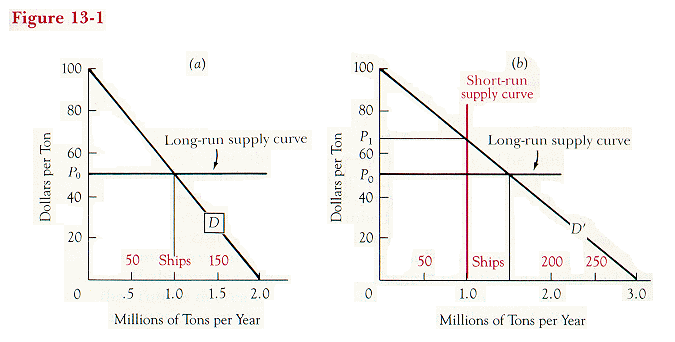
Supply and demand curves for shipping, showing the effect of an unanticipated increase in demand. Figure 13-la shows the situation before the increase and Figure 13-lb after. The horizontal axis shows both quantity of cargo carried each year and the equivalent number of ships. The short-run supply curve is vertical at the current number of ships (and amount of cargo they carry). The long-run supply curve is horizontal at the cost of producing shipping (the annualized cost of building a ship divided by the number of tons it carries).
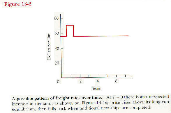
Shipyards immediately start building new ships. At the end of a year, the new ships are finished and the price drops back down to the old level. Figure 13-2 shows the sequence of events in the form of a graph of price against time.
Looking again at Figure 13-lb, note that it has two supply curves--a vertical short-run supply curve and a horizontal long-run supply curve. No ships can be built in less than a year, so there is no way a high price can increase the supply of shipping in the short run. Since operating costs are, by assumption, zero, it pays shipowners to operate the ships however low the price; there is no way a low price can reduce the supply of shipping in the short run. So in the short run, quantity supplied is independent of price for any price between zero and infinity.
The situation in the long run is quite different. At any price where ships more than cover their construction cost, it pays to build ships; so in the long run, the industry will produce an unlimited quantity of shipping at any price above P0 = $50/ton. As ships are built, the short-run supply curve shifts out. At any price below P0, building a ship costs more than the ship is worth, so quantity supplied falls as the existing ships wear out. So the long-run supply curve is horizontal. It is worth noting that on the "up" side--building ships--the long run is a good deal shorter than on the "down" side.
Suppose that instead of the increase in demand shown in Figure 13-1b, there is instead a decrease in demand, from D to D", as shown in Figure 13-3a. Price drops. Since there are no operating costs, existing ships continue to carry cargo as long as they get any price above zero. The price is at the point where the old (short-run) vertical supply curve intersects the new demand curve (A).
Building a ship is now unprofitable, since it will not, at the new price, repay its construction costs. No ships are built. Over the next five years, 25 ships wear out, bringing the long-run quantity supplied (and the short-run supply curve) down to a point where the price is again $50/ton (B). Figure 13-3b shows how the price and the number of ships change with time.
There is one thing wrong with this story. The initial equilibrium assumed that the price of shipping was going to stay the same over the lifetime of a ship--that was why ships were produced if and only if the return at current prices, multiplied by the lifetime of the ship, totaled at least the cost of production. The later developments assumed that the demand curve, and hence the price, could vary unpredictably.
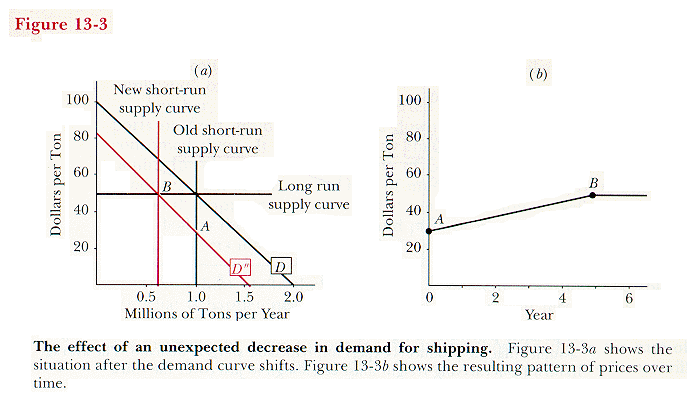
The effect of an unexpected decrease in demand for shipping. Figure 13-3a shows the situation after the demand curve shifts. Figure 13-3b shows the resulting pattern of prices over time.
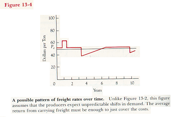
A possible pattern of freight rates over time. Unlike Figure 13-2, this figure assumes that the producers expect unpredictable shifts in demand. The average return from carrying freight must be enough to just cover the costs.
If shipowners expect random changes in future demand and believe that future decreases will be at least as frequent and as large as future increases, the price at which they are just willing to build will be more than $50/ton. Why? Because ships can be built quickly, so that the gain from an increase in demand is short-lived, but wear out slowly, so that the loss from a decrease in demand continues for a long time. Compare the short period of high prices in Figure 13-2 with the long period of low prices in Figure 13-3b. If the current price is high enough (Pe on Figure 13-4) that any increase causes ships to be built, then an increase in demand will hold prices above Pe for only a year. A decrease can keep prices below Pe for up to twenty years. If Pe were equal to $50/ton, the price at which ships exactly repay the cost of building them, the average price would be lower than that and ships, on average, would fail to recover their costs. So Pe must be above $50/ton.
This is the same point that I made earlier in describing the effect of sunk costs in the widget industry. In order to make the behavior of the shipowners rational, we must assume that they do not start building ships until the price is high enough that the profits if demand does not fall make up for the losses if it does. The pattern of price over time in the industry then looks something like Figure 13-4.
A True Story
Many years ago, while spending a summer in Washington, I came across an interesting piece of economic analysis involving these principles. The congressman I was working for had introduced a bill that would have abolished a large part of the farm program, including price supports for feed grains (crops used to feed animals). Shortly thereafter the agriculture department released a "study" of the effects of abolishing those particular parts of the farm program. Their conclusion, as I remember, was that farm income would fall by $5 billion while the government would save only $3 billion in reduced expenditure, for a net loss of $2 billion.
The agriculture department's calculations completely ignored the effect of the proposed changes on consumers--although the whole point of the price support program was (and is) to raise the price of farm products and thus of food. Using the agriculture department's figures, the proposed abolition would have saved consumers (as I remember) about $7 billion, producing a net gain of $5 billion. The agriculture department, which of course opposed the proposed changes, failed to mention that implication of its analysis.
Another part of the report asserted that the abolition of price supports on feed grains would drive down the prices of the animals that consumed them. It went on to say that the price drop would first hit poultry producers, then producers of pork and lamb, and finally beef producers. All of this, to the best of my knowledge, is correct. The conclusion that appears to follow is that poultry producers will be injured a great deal by the abolition, lamb and pork producers somewhat less, and beef producers injured least of all. This is almost the precise opposite of the truth.
If you think about the situation for a moment, you should be able to see what is happening. Removing price supports on feed grains lowers the cost of production for poultry, pork, lamb, and beef--feed grains are probably the largest input for producing those foods. In the case of poultry, the flocks can be rapidly increased, so the poultry producers will receive an above-normal profit (cost of production has fallen, price of poultry has not) for only a short time. Once the flocks have increased, the price of chickens falls and the return to their producers goes back to normal. The herds of pigs and sheep take longer to increase, so their producers get above-normal returns for a longer period, and the beef producers get them for longer still. The situation is just like the situation of the shipowners when demand increases, except that there is a drop in production cost rather than an increase in the demand schedule. The agriculture department appeared to be saying that the beef producers would receive the least injury and the poultry producers the greatest injury from the proposed change; what their analysis actually implied was that the beef producers would receive the largest benefit and the poultry producers the smallest benefit.
PART 2 - LONG-RUN
AND
SHORT-RUN COSTS
So far, we have been analyzing the influence of uncertainty on prices by taking account of the effect of sunk costs on the behavior of profit-maximizing firms. A more technical description of what we are doing is that we are analyzing the effect of uncertainty in terms of Marshallian quasi-rents-- "Marshallian" because this approach, along with much of the rest of modern economics, was invented by Alfred Marshall about a hundred years ago and "quasi-rents" because the return on sunk costs is in many ways similar to the rent on land. Both can be viewed as the result of a demand curve intersecting a perfectly inelastic supply curve--although in the case of sunk costs, the supply curve is inelastic only in the short run.
The more conventional way of analyzing these questions is in terms of short-run and long-run cost curves and the resulting short-run and long-run supply curves. I did not use that approach in Chapter 9, where supply curves were deduced from cost curves, and so far I have not used it here. Why?
The reason for ignoring the distinction between long-run and short-run costs in Chapter 9 was explained there; in the unchanging world we were analyzing, long run and short run are the same. The reason I did not introduce the ideas of this chapter in that form is that the way in which I did introduce it provides a more general and more powerful way of analyzing the same questions. It is more general because it allows us to consider productive assets--such as ships and factories--with a variety of lifetimes and construction times, not merely the extreme (and arbitrary) classes of "short-" and "long-" lived. It is more powerful because it not only gives us the long-run and short-run supply curves but also shows what happens in between, both to the price of the productive assets and to the price of the goods they produce.
The simplest way to demonstrate all of this--and to prepare you for later courses that will assume you are familiar with the conventional approach--is to work out the short-run/long-run analysis as a special case of the approach we have been following. While doing so, we will also be able to examine some complications that have so far remained hidden behind the simplifying assumptions of our examples.
We start with an industry. Since we used up our quota of widgets earlier in the chapter, we will make it the batten industry. Battens are produced in batten factories. There are many batten firms, so each is a price taker. A firm entering the industry--or a firm already in the industry that is replacing a worn-out factory--must choose what size factory to build. A small factory is inexpensive to build but expensive to operate--especially if you want to produce a large amount of output. Larger factories cost more to build but are more efficient for producing large quantities. A firm can only operate one factory at a time.
Figures 13-5 through 13-7 show the cost curves for three different factories. The first costs $1 million to build, the second $3 million, and the third $5 million. A factory has no scrap value, so the investment is a sunk cost. Each factory lasts ten years. The interest rate is zero, so the annual cost associated with each factory is one tenth the cost of building it. One could easily enough do the problem for a more realistic interest rate, but that would complicate the calculations without adding anything important.
Total cost is the sum of fixed cost and variable cost. The figures are drawn on the assumption that the only fixed cost in producing battens is the cost of building the factory; all other costs are variable. Since this implies that the fixed cost and the sunk cost are identical, so are variable cost (total cost minus fixed cost) and recoverable cost (total cost minus sunk cost). The figures show average variable cost (AVC); it might just as well have been labeled ARC for "average recoverable cost."
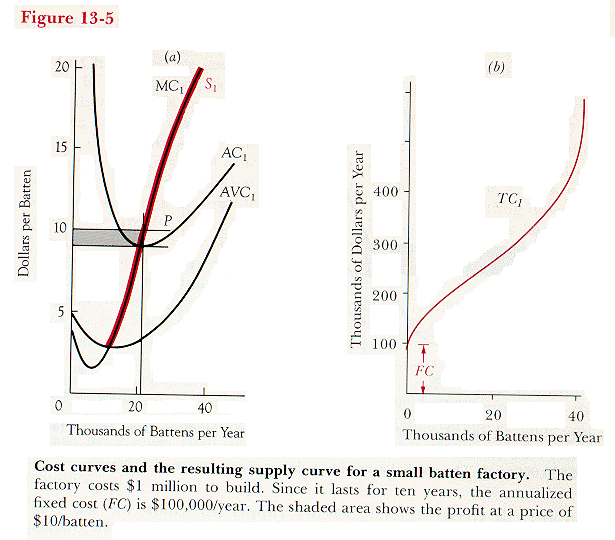
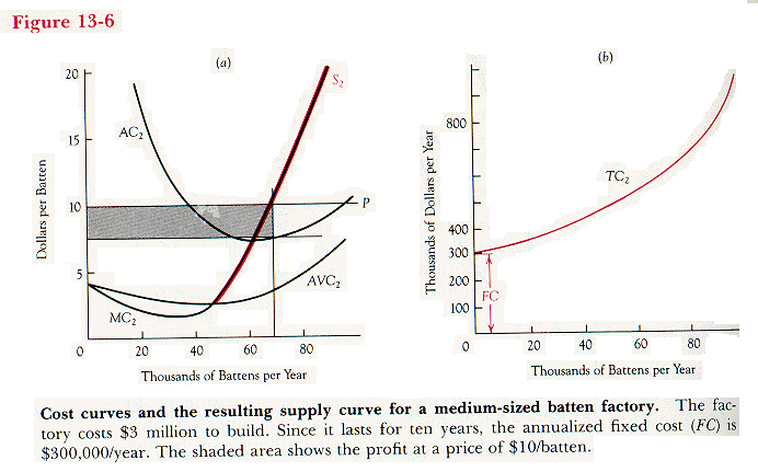
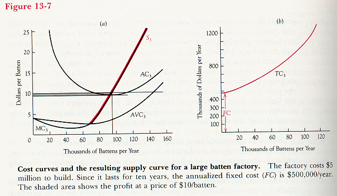
Each pair of figures shows four cost curves--total cost (TC), marginal cost (MC), average cost (AC), and average variable cost (AVC). Total cost includes the (annualized) cost of the factory; since that is assumed to be the only fixed cost, total cost at a quantity of zero is the annualized cost of the factory--$100,000/year on Figure 13-5b. Since average cost is defined as total cost over quantity, it too includes the cost of the factory. Average variable cost, on the other hand, does not include the cost of the factory, since that is fixed.
So far as marginal cost is concerned, it does not matter whether or not we include the cost of the factory. Marginal cost is the slope of total cost; adding a constant term to a function simply shifts it up without affecting its slope.
Suppose the batten firm has built the factory of Figure 13-5. The market price of a batten is P; the firm must decide how many to produce each year. Just as in Chapter 9, the firm maximizes its profit by producing the quantity for which MC = P, provided that at that quantity it is not losing money.
In Chapter 9, we could see whether the firm was making or losing money by comparing price to average cost; if average cost is greater than price, then profit is negative and the firm should go out of business. This time we have two average costs--AC and AVC. Which should we use?
We should use AVC. The firm already has the factory; it is deciding whether or not to shut it down. If the firm shuts down the factory, it will not get back the money that was spent to build it--that is a sunk cost. What it will save is its variable cost. If the savings from shutting down the factory are greater than the loss from no longer having any battens to sell, then the factory should be shut down. Otherwise it should continue to operate. So as long as price is greater than average variable cost, the firm continues to operate the factory, producing the quantity for which marginal cost equals price. If price is lower than average cost, the factory is not paying back its cost of construction and should never have been built--but it is too late to do anything about that. Sunk costs are sunk costs.
The curves labeled S1-S3 on Figures 13-5 through 13-7 are the supply curves implied by the previous two paragraphs. Each S runs along the marginal cost curve, starting at its intersection with average variable cost. For any price lower than that, quantity supplied is zero.
These are the short-run supply curves. They correctly describe the behavior of a firm that already owns a functioning factory. But in the long run, factories wear out and must be replaced. A firm that is about to build a factory is in a different situation, in two respects, from a firm that already has a factory. First, the cost of building the factory is not yet sunk--the firm has the alternative of not building and not producing. The firm will build only if it expects price to be above average cost--including in the average the cost of building the factory.
The second difference is that a firm about to build can choose which size of factory it prefers. Its choice will depend on what the price is. So the long-run supply curve must take account of the relation between the price of battens and the size of the factories in which they will be produced.
How do we find the long-run supply curve of a firm? We consider a firm that is about to build a factory and expects the market price of battens to remain at its present level for at least the next ten years--the lifetime of the factory. The firm's long-run supply curve is then the relation between the quantity the firm chooses to produce and the price.
We solve the problem in two steps. First we figure out, for each size of factory, how many battens the firm will produce if it decides to build a factory of that size. Then we compare the resulting profits, in order to find out which factory the firm will choose to build. Once we know which factory the firm chooses to build and how much a firm with a factory of that size chooses to produce, we know quantity supplied at that price. Repeat the calculation for all other prices and we have the firm's long-run supply curve.
Figures 13-5 through 13-7 show the calculations for a price of $10/batten. As we already know, if a price-taking firm produces at all, it maximizes its profit by producing a quantity for which MC = P. So for each size of factory, a firm that chose to build that factory would produce the quantity for which marginal cost was equal to price.
Having done so, what would the firm's profit be? Profit per unit is simply price minus average cost. The firm should include the cost of building the factory in deciding which factory to build, so the relevant average is average cost, not average variable cost. Total profit is profit per unit times number of units--the shaded rectangle in each figure. It is largest for Figure 13-6, so the firm builds a $3 million factory and produces that quantity for which, in such a factory, price equals marginal cost.
Figure 13-8 shows the result of repeating the calculations for many different prices. As I have drawn the curves, the less expensive factories have a lower average cost for low levels of output and a higher average cost for high levels. The result is that as price (and quantity) increase, so does the optimal size of the factory. The long-run supply curve for the firm (Figure 13-8b) is then pieced together from portions of the short-run supply curves of Figures 13-5 through 13-7. In doing so, we limit ourselves to the part of each short-run supply curve above the corresponding average cost (AC not AVC), since that is the long-run supply curve for that size of factory. We end up with the long-run supply curve for a firm that is free to vary factory size as well as other inputs.
Looking at Figure 13-8b, we see that the smallest size of factory is irrelevant to the firm's supply curve, since there is no price of battens at which it would be worth building such a factory. If the market price is below P0, none of the three sizes of factory can make enough money to justify the cost of building it, so the firm produces nothing. For prices between P0 and P1 on Figure 13-8b, the firm maximizes its profit by building a $3 million factory and producing the quantity for which the marginal cost (MC2 on Figure 13-6a) equals the price. For prices above P1, it does better building a $5 million factory and producing along the MC3 curve of Figure 13-7a. So S is the firm's long-run supply curve.
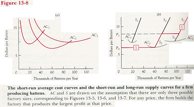
An alternative way of deriving the long-run supply curve of the firm is to consider the factory itself as one more input in the production function. Just as in Chapter 9, one then calculates the lowest cost bundle of inputs for each level of output; the result tells you, for any quantity of output, how much it costs to produce and what inputs--including what size of factory--you should use. You then go on to calculate average cost (the same curve shown on Figure 13-8a), marginal cost, and the supply curve. Since we are considering the long-run supply curve, we are (temporarily) back in the unchanging world of Chapters 1-11.
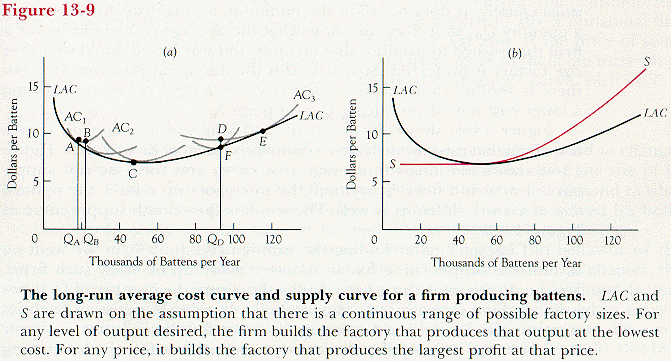
Figure 13-9a shows what the firm's long-run average cost curve would be like if, instead of limiting the firm to only three sizes of factory, we allowed it to choose from a continuous range of factory sizes. The solid line LAC on the figure is the resulting long-run average cost curve; the gray lines are average cost curves for several different factory sizes, including those shown on Figures 13-5 through 13-7. Since for any quantity, the firm chooses that factory size which produces that quantity at the lowest possible cost, the average cost curve for a factory can never lie below the average cost curve for the firm. Every point on the firm's long-run average cost curve is also on the average cost curve for some size of factory--the size the firm chooses to build if it expects to produce that quantity of output. The result is what you see on Figure 13-9a; the average cost curves for the different factory sizes lie above the firm's long-run average cost curve and are tangent to it.
One feature of figures such as 13-9a that some people find puzzling is that the point where a factory average cost curve touches the firm's long-run average cost curve is generally not at the minimum average cost for that size of factory. AC1, for example, touches LAC not at point B, which is its minimum, but at point A, and similarly for all the others except AC2. Mathematically, the reason for this is quite simple. AC1 is tangent to LAC at point A. At the point of tangency, the two curves have the same slope. Unless LAC is at its minimum--as it is at point C, where it touches AC2--its slope is not zero. Since the slope of LAC is not zero at the point of tangency, neither is the slope of AC1; so AC1 cannot be at its minimum. The same applies to all of the points of tangency except C.
As I have commented before, one can read through a proof without ever understanding why the conclusion is correct; for some of you, the previous paragraph may be an example of that. Another way of putting the argument is to point out that while the firm that chooses to produce quantity QA could lower its average cost by expanding output to QB, it would then be producing a larger quantity; if it wished to produce that quantity, it could do so at an even lower average cost by using a bigger factory. B shows the minimum average cost for producing in a $1 million factory. It does not show the minimum average cost for producing a quantity QB, so it does not show what the average cost would be for a firm that wished to produce that quantity and was free to build whatever size factory it preferred. Similarly, D is the minimum point on AC3, but there is another (unlabeled) average cost curve lying below it, providing a lower cost way of producing QD--at point F.
Figure 13-9a shows the short-run and long-run average cost curves for a firm that can choose from a continuous range of factory sizes. Figure 13-9b shows the long-run average cost curve and the long-run supply curve for such a firm. Every time the price goes up a little, the optimal size of factory shifts up as well. The result is the smooth supply curve of Figure 13-9b.
In Chapter 9, after finding the supply curve for a firm, we went on to find the supply curve for an industry made up of many such firms. We can do the same thing here. In the short run, the number of factories is fixed; there is not enough time to build more or for existing factories to wear out. So the short-run supply curve for the industry is simply the horizontal sum of the short-run supply curves for all the existing factories--just as in the case of the competitive industry with closed entry discussed in Chapter 9.
In the long run, the number of factories can vary; firms may build new factories or fail to replace existing factories as they wear out. Unless there are barriers to entry, such as laws against building new factories, we are in the second case of Chapter 9--a competitive industry with free entry. If the inputs to the industry are in perfectly elastic supply so that their price does not depend on industry output, the (constant-cost) industry's long-run supply curve is S on Figure 13-10--a horizontal line at price = marginal cost = minimum average cost. If the price of some of the inputs rises as the industry purchases more of them (an increasing-cost industry), the result is an upward-sloped supply curve, such as S'.
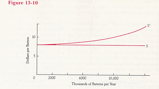
Two possible long-run supply curves for the batten industry. S, which is horizontal at a price equal to minimum average cost, is drawn on the assumption that inputs are available in perfectly elastic supply. S' is drawn on the assumption that as quantity increases, input prices are bid up.
Part 1 vs Part 2--Two Approaches
Compared
The short-run supply curve tells us how the firm will respond to changes in price over periods too short to make it worth changing the size of its factory; the long-run supply curve tells how the firm will respond to what it regards as permanent changes in price. We have now solved for both. In doing so, what have we learned that we did not already know?
The most important lesson is how to calculate the behavior of the firm over the short run. In all of the earlier examples of this chapter, the firms had simple all-or-none patterns of production. A widget factory either produced at capacity or shut down; a ship continued to carry a full load of freight as long as it got anything at all for doing so. We were, in effect, assuming the cost curves shown in Figures 13-11a and 13-11b--marginal cost constant up to some maximum level of production and infinite beyond that. We were also assuming that there was only one kind of factory and one kind of ship.
In analyzing the batten factory, we allowed for more realistic cost curves. By doing so, we saw how, even in the short run, quantity supplied can vary continuously with price. We could have done the same thing in the earlier analysis; I chose not to. All-or-none production was a simplifying assumption used to avoid complications that were, at that point, inessential. The discussion of long-run and short-run supply curves was a convenient point at which to drop that simplification.
What are the disadvantages of the short-run/long-run approach? One of them is that it encourages students to confuse sunk costs and fixed costs. In the examples that are used, the two are generally the same, but there is no reason why they have to be.
In the batten industry, as I pointed out earlier, the curve labeled average variable cost could also have been labeled average recoverable cost, since the two are equal. I labeled it AVC in deference to convention; that is how you will generally see it in other textbooks. It would have been more correct to have labeled it ARC. It is the fact that the cost is recoverable, not the fact that it is variable, that is essential to the way in which the curve is related to the short-run supply curve. If we were considering a situation in which variable cost and recoverable cost were not the same, we could have simply drawn the ARC curve and forgotten about AVC.
One of the faults of the short-run/long-run approach is that it encourages confusion between fixed and sunk costs. One of its limitations is that it distinguishes between only two kinds of costs--short-run and long-run. The more general approach to sunk cost, which we developed earlier in the chapter, can be used to analyze a much broader range of situations, including ones in which there are several long-lived productive assets with different lifetimes.

A second limitation is that the short-run/long-run approach says nothing about what happens to price between the two periods--how it adjusts over time to unexpected changes in demand. If we know how many factories of what size exist, the short-run supply curve allows us to calculate price and quantity; whether or not we know how many factories exist, the long-run supply curve tells us what price and quantity must eventually be if the situation remains stable for long enough. But the approach does not explain how to calculate the path by which price and quantity move from the one value to the other--which is one of the things we did in analyzing the widget and shipping industries.
None of this means that the short-run/long-run approach is wrong. Both in using economics and in teaching it, one must balance the costs and benefits of different degrees of simplicity. The short-run/long-run approach described in this section has the advantages and the disadvantages of greater simplicity; it is easier to teach but tells us less of what we want to know than the approach used earlier in the chapter.
In one sense, the difference is entirely pedagogical. Once you understand either approach, you can develop the other out of it. Starting with short- and long-run cost curves, you could, with a little ingenuity, figure out how to analyze more complicated cases or how to trace the path of price and quantity over time. Starting with sunk costs, you can work out short-run and long-run cost curves as special cases--not only in the shipping industry of Figures 13-l through 13-4 but in more complicated situations as well. By teaching the material in both ways, I hope I have allowed you to learn it in whichever way you found more natural. That is a benefit. Its cost is measured in additional pages of book and additional hours of time--mine in writing and yours in reading. The production of textbooks involves the same sort of trade-off between costs and benefits as does the production of anything else--or any other action requiring choice.
PART 3 - SPECULATION
It is difficult to read either newspapers or history books without occasionally coming across the villainous speculators. Speculators, it sometimes seems, are responsible for all the problems of the world--famines, currency crises, high prices.
A speculator buys things when he thinks they are cheap and sells them when he thinks they are expensive. Imagine, for example, that you decide there is going to be a bad harvest this year. If you are right, the price of grain will go up. So you buy grain now, while it is still cheap. If you are right, the harvest is bad, the price of grain goes up, and you sell at a large profit.
There are several reasons why this particular way of making a profit gets so much bad press. For one thing, the speculator is, in this case at least, profiting by other people's bad fortune, making money from, in Kipling's phrase, "Man's belly pinch and need." Of course, the same might be said of farmers, who are usually considered good guys. For another, the speculator's purchase of grain tends to drive up the price, making it seem as if he is responsible for the scarcity.
But in order to make money, the speculator must sell as well as buy. If he buys when grain is plentiful, he does indeed tend to increase the price then; but if he sells when it is scarce (which is what he wants to do in order to make money), he increases the supply and decreases the price just when the additional grain is most useful.
A different way of putting it is to say that the speculator, acting for his own selfish motives, does almost exactly what a benevolent despot would do. When he foresees a future scarcity of wheat, he induces consumers to use less wheat now. The speculator gets consumers to use less wheat now by buying it (before the consumers themselves realize the harvest is going to be bad), driving up the price; the higher price encourages consumers to consume less food (by slaughtering meat animals early, for example, to save their feed for human consumption), to import food from abroad, to produce other kinds of food (go fishing, dry fruit, . . .), and in other ways to prepare for the anticipated shortage. He then stores the wheat and distributes it (for a price) at the peak of the famine. Not only does he not cause famines, he prevents them.
More generally, speculators (in many things, not just food) tend, if successful, to smooth out price movements, buying goods when they are below their long-run price and selling them when they are above it, raising the price towards equilibrium in the one case and lowering it towards equilibrium in the other. They do what governmental "price-stabilization" schemes claim to do--reduce short-run fluctuations in prices. In the process, they frequently interfere with such price-stabilization schemes, most of which are run by producing countries and designed to "stabilize" prices as high as possible.
Why indeed should we welcome you, Master Stormcrow? Lathspell I name you, ill-news; and ill news is an ill guest they say.
--Grima to Gandalf in The Two Towers by J.R.R. Tolkien
At least part of the unpopularity of speculators and speculation may reflect the traditional hostility to bearers of bad news; speculators who drive prices up now in anticipation of a future bad harvest are conveying the fact of future scarcity and are forcing consumers to take account of it. Part also may be due to the difficulty of understanding just how speculation works. Whatever the reason, ideas kill, and the idea that speculators cause shortages must be one of the most lethal errors in history. If speculation is unpopular it is also difficult, since the speculator depends for his profit on not having his stocks of grain seized by mob or government. In poor countries, which means almost everywhere through almost all of history, the alternative to speculation in food crops is periodic famine.
One reason people suspect speculators of causing price fluctuations is summarized in the Latin phrase cui bono; a loose translation would be "Who benefits?" If the newspapers discover that a gubernatorial candidate has been receiving large campaign donations from a firm that made $10 million off state contracts last year, it is a fair guess that the information was fed to them by his opponent. If a coup occurs somewhere in the Third World and the winners immediately ally themselves with the Soviet Union (or the United States), we do not have to look at the new ruler's bank records to suspect that the takeover was subsidized by Moscow (or Washington).
While cui bono is a useful rule for understanding many things, it is not merely useless but positively deceptive for understanding price movements. The reason is simple. The people who benefit from an increase in the price of something are those who produce it, but by producing, they drive the price not up but down. The people who benefit by a price drop are those who buy and consume the good, but buying a good tends to increase its price, not lower it. The manufacturer of widgets may spend his evenings on his knees praying for the price of widgets to go up, but he spends his days behind a desk making it go down. Hence the belief that price changes are the work of those who benefit by them is usually an error and sometimes a dangerous one.
Speculators make money by correctly predicting price changes, especially those changes that are difficult to predict. It is natural enough to conclude, according to the principle of cui bono, that speculators cause price fluctuations.
The trouble with this argument is that in order to make money, a speculator must buy when prices are low and sell when they are high. Buying when prices are low raises low prices; selling when prices are high lowers high prices. Successful speculators decrease price fluctuations, just as successful widget makers decrease the price of widgets. Destabilizing speculators are, of course, a logical possibility; they can be recognized by the red ink in their ledgers. The Hunt brothers of Texas are a notable recent example. A few years ago, they lost several billion dollars in the process of driving the price of silver up to what turned out to be several times its long-run equilibrium level.
It is true, of course, that a speculator would like to cause instability, supposing that he could do so without losing money; more precisely, he would like to make the prices of things he is going to sell go up before he sells them and of things he is going to buy go down before he buys them. He cannot do this by his market activities, but he can try to spread misleading rumors among other speculators; and, no doubt, some speculators do so. His behavior in this respect is like that of a producer who advertises his product; he is trying to persuade people to buy what he wants to sell. The speculator faces an even more skeptical audience than the advertiser, since it is fairly obvious that if he really expected the good to go up he would keep quiet and buy it himself. So the private generating of disinformation, while it undoubtedly occurs, is unlikely to be very effective.
I once heard a talk by an economist who had applied the relationship between stabilization and profitable speculation in reverse. The usual argument is that speculators, by trying to make a profit, provide the useful public service of stabilizing prices. The reverse argument involved not private speculators but central banks. Central banks buy and sell currencies, supposedly in order to stabilize exchange rates (an exchange rate is the price of one kind of money measured in another). They are widely suspected (by economists and speculators) of trying to keep exchange rates not stable but above or below their market clearing levels.
If profitable speculation is stabilizing, one might expect successful stabilization of currencies to be profitable. If the banks are buying dollars when they are temporarily cheap and selling them when they are temporarily expensive, they should be both stabilizing the value of the dollar and making a profit. One implication of this argument is that the central banks are superfluous--if there are profits to be made by stabilizing currencies, speculators will be glad to volunteer for the job. A second implication is that we can judge the success of central banks by seeing whether they in fact make or lose money on their speculations. The conclusion of the speaker, who had studied precisely that question, was that they generally lost money.
OPTIONAL SECTION
CHOICE
IN
AN UNCERTAIN WORLD
In Chapters 1-11, we saw how markets work to determine prices and quantities in a certain and unchanging world. In Chapter 12, we learned how to deal with a world that was changing but certain. In such a world, any decision involves a predictable stream of costs and benefits--so much this year, so much next year, so much the year after. One simply converts each stream into its present value and compares the present values of costs and benefits, just as we earlier compared annual flows of costs and benefits.
The next step is to analyze individual choice in an uncertain world. Again our objective is to convert the problem we are dealing with into the easier problem we have already solved. To describe an uncertain world, we assume that each individual has a probability distribution over possible outcomes. He does not know what will happen but he knows, or believes he knows, what might happen and how likely it is to happen. His problem, given what he knows, is how to achieve his objectives as successfully as possible.
Consider, for example, an individual betting on whether a coin will come up heads or tails. Assuming the coin is a fair one, half the time it will come up heads and half the time tails. The gambler's problem is to decide what bets he should be willing to take.
The answer seems obvious--take any bets that offer a payoff of more than $1 for each $1 bet; refuse any that offer less. If someone offers to pay you $2 if the coin comes up heads, on condition that you pay him $1 if it comes up tails, then on average you gain by accepting the bet and should do so. If he offers you $0.50 for the risk of $1, then on average you lose by accepting; you should refuse the bet.
In these examples, you are choosing between a certain outcome (decline the bet--and end up with as much money as you started with) and an uncertain outcome (accept the bet--end up with either more or less). A more general way of putting the rule is that in choosing among alternatives, you should choose the one that gives you the highest expected return, where the expected return is the sum of the returns associated with the different possible outcomes, each weighted by its probability.
Maximizing Expected Return. This is the correct answer in some situations but not in all. If you make a fifty-fifty bet many times, you are almost certain to win about half the time; a bet that on average benefits you is almost certain to give you a net gain in the long term. If, for instance, you flip a fair coin 1,000 times, there is only a very small chance that it will come up heads more than 600 times or fewer than 400. If you make $2 every time it comes up heads and lose $1 every time it comes up tails, you are almost certain, after 1,000 flips, to be at least $200 ahead.
The case of the gambler who expects to bet many times on the fall of a coin can easily be generalized to describe any game of chance. The rule for such a gambler is "Maximize expected return." Since we defined expected return as the sum, over all of the possible outcomes, of the return from each outcome times the probability of that outcome, we have:
<R> ![]() piRi. (Equation 1)
piRi. (Equation 1)
Here pi is the probability of outcome number i occurring, Ri is the return from outcome number i, and <R> is the expected return.
When you flip a coin, it must come up either heads or tails; more generally, any gamble ends up with some one of the alternative outcomes happening, so we have:
![]() pi
= 1. (Equation 2)
pi
= 1. (Equation 2)
In the gamble described earlier, where the gambler loses $1 on tails and gains $2 on heads, we have:
p1 = 0.5; R1 = + $2 (heads)
p2 = 0.5; R2 = - $1 (tails)
<R> = (p1 x R1) + (p2 x R2) = [0.5 x (+ $2)] + [0.5 x ( - $1) ]= + $0.50.
Here p1 and p2, the probabilities of heads and tails respectively, are each equal to one half; your expected return is $0.50. If you play the game many times, you will on average make $0.50 each time you play. The expected return from taking the gamble is positive, so you should take it--provided you can repeat it many times. The same applies to any other gamble with a positive expected return. A gamble with an expected return of zero--you are on average equally well off whether or not you choose to take it--is called a fair gamble.
We now know how a gambler who will take the same gamble many times should behave. In choosing among several gambles, he should take the one with the highest expected return. In the particular case where he is accepting or declining bets, so that one of his alternatives is a certainty of no change, he should take any bet that is better than a fair gamble.
Maximizing Expected Utility. Suppose, however, that you are only playing the game once--and that the bet is not $1 but $50,000. If you lose, you are destitute--$50,000 is all you have. If you win, you gain $100,000. You may feel that a decline in your wealth from $50,000 to zero hurts you more than an increase from $50,000 to $150,000 helps you. One could easily enough imagine situations in which losing $50,000 resulted in your starving to death while gaining $100,000 produced only a modest increase in your welfare.
Such a situation is an example of what we earlier called declining marginal utility. The dollars that raise you from zero to $50,000 are worth more per dollar than the additional dollars beyond $50,000. That is precisely what we would expect from the discussion of Chapter 4. Dollars are used to buy goods; we expect goods to be worth less to you the more of them you have.
When you choose a profession, start a business, buy a house, or stake your life savings playing the commodity market, you are betting a large sum, and the bet is not one you will repeat enough times to be confident of getting an average return. How can we analyze rational behavior in such situations?
The answer to this question was provided by John Von Neumann, the same mathematician mentioned in Chapter 11 as the inventor of game theory. He demonstrated that by combining the idea of expected return used in the mathematical theory of gambling (probability theory) with the idea of utility used in economics, it was possible to describe the behavior of individuals dealing with uncertain situations--whether or not the situations were repeated many times.
The fundamental idea is that instead of maximizing expected return in dollars, as in the case described above, individuals maximize expected return in utiles--expected utility. Each outcome i has a utility Ui. We define expected utility as:
<U> ![]()
![]() piUi.
(Equation 3)
piUi.
(Equation 3)
Your utility depends on many things, of which the amount of money you have is only one. If we are considering alternatives that only differ with regard to the amount of money you end up with, we can write:
Ui = U(Ri).
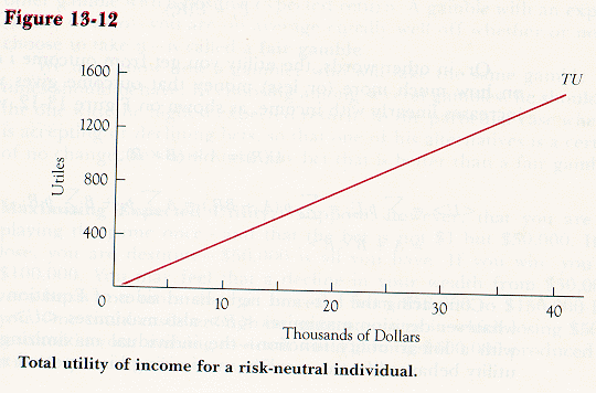
Or, in other words, the utility you get from outcome i depends only on how much more (or less) money that outcome gives you. If utility increases linearly with income, as shown on Figure 13-12, we have:
U(R) = A + (B x R);
<U> =![]() piUi =
piUi =![]() pi(A + BRi) =A
pi(A + BRi) =A![]() pi + B
pi + B ![]() piRi =
piRi =
= A + B<R>. (Equation 4)
Comparing the left and right-hand sides of Equation 4, we see that whatever decision maximizes <R> also maximizes <U>. In this case--with a linear utility function--the individual maximizing his expected utility behaves like the gambler maximizing his expected return.
A Methodological Digression. In going from gambling games to utility graphs, we have changed somewhat the way in which we look at expected return. In the case of gambling, return was defined relative to your initial situation--positive if you gained and negative if you lost. That was a convenient way of looking at gambling because the gambler always has the alternative of refusing to bet and so ending up with a return of zero. But in an uncertain world, the individual does not usually have that alternative; sometimes--indeed almost always--he is choosing among alternatives all of which are uncertain. In that context, it is easier to define zero return as ending up with no money at all and to measure all other outcomes relative to that. We can then show the utility of any outcome on a graph such as Figure 13-12 as the utility of the income associated with that outcome. If you start with $10,000 and bet all of it at even odds on the flip of a coin--heads you win, tails you lose--then the utility to you of the outcome "heads" is the utility of $20,000. The utility to you of the outcome "tails" is the utility of zero dollars.
A second difficulty with Figure 13-12 is the ambiguity as to just what is being graphed on the horizontal axis--what is utility a function of? Is it income (dollars per year) or money (dollars)? Strictly speaking, utility is a flow (utiles per year) that depends on a flow of consumption (apples per year). The utility we get by consuming 100 apples, or whatever else we buy with our income, depends in part on the period of time over which we consume them.
If I were being precise, I would do all the analysis in terms of flows and compare alternatives by comparing the present values of those flows, in dollars or utiles. This would make the discussion a good deal more complicated without adding much to its content. It is easier to think of Figure 13-12, and similar figures, as describing either someone who starts with a fixed amount of money and is only going to live for a year, or, alternatively, someone with a portfolio of bonds yielding a fixed income who is considering gambles that will affect the size of his portfolio. The logic of the two situations is the same. In the one case, the figure graphs the utility flow from a year's expenditure; in the other case, it graphs the present value of the utility flow from spending the same amount every year forever. Both approaches allow us to analyze the implications of uncertainty while temporarily ignoring other complications of a changing world. To make the discussion simpler, I will talk as if we are considering the first case; that way I can talk in "dollars" and "utiles" instead of "dollars per year" and "utiles per year." The amount of money you have may still sometimes be described as your income--an income of x dollars/year for one year equals x dollars.
Risk
Preference and the Utility
Function
Or
As I Was Saying When I So Rudely
Interrupted Myself
Figure 13-12 showed utility as a linear function of income; Figure 13-13a shows a more plausible relation. This time, income has declining marginal utility. Total utility increases with income, but it increases more and more slowly as income gets higher and higher.
Suppose you presently have $20,000 and have an opportunity to bet $10,000 on the flip of a coin at even odds. If you win, you end up with $30,000; if you lose, you end up with $10,000.
In deciding whether to take the bet, you are choosing between two different gambles. The first, the one you get if you do not take the bet, is a very simple gamble indeed--a certainty of ending up with $20,000. The second, the one you get if you do take the bet, is a little more complicated--a 0.5 chance of ending up with $10,000 and a 0.5 chance of ending up with $30,000. So for the first gamble, we have:
p1 = 1; Rl = $20,000; U1 = U(R1) = U($20,000) = 1,000 utiles (from Figure 13-13a)
<U> = p1 x U1 = 1,000 utiles.
For the second gamble, we have:
p1 = 0.5; R1 = $10,000; U1 = U(R1) = U($10,000) = 600 utiles (from Figure 13-13a)
p2 = 0.5; R2 = $30,000; U2 =U(R2) = U($30,000) = 1,200 utiles (from Figure 13-13a)
<U> = (p1 x U1) + (p2 x U2) = (0.5 x 600 utiles) + (0.5 x 1,200 utiles) = 900 utiles.
The individual takes the alternative with the higher expected utility; he declines the bet. In money terms, the two alternatives are equally attractive; they have the same expected return. In that sense, it is a fair bet. In utility terms, the first alternative is superior to the second. You should be able to convince yourself that as long as the utility function has the shape shown in Figure 13-13a, an individual will always prefer a certainty of $1 to a gamble whose expected return is $1.
An individual who behaves in that way is risk averse. A utility function that is almost straight, such as Figure 13-13b, represents an individual who is only slightly risk averse. Such an individual would decline a fair gamble but might accept one that was a little better than fair--bet $1,000 against $1,100 on the flip of a coin, for example. An individual who was extremely risk averse (Figure 13-13c) might still accept a gamble--but only one with a very high expected return, such as risking $1,000 on the flip of a coin to get $10,000.
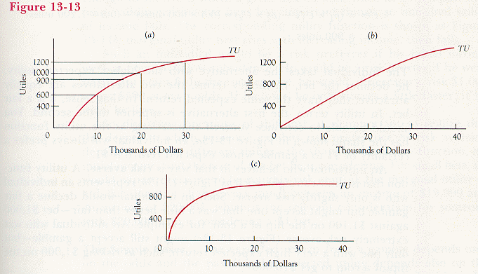
Total utility of income for a risk-averse individual. Figure 13-13b corresponds to an individual who is only slightly risk averse; he will refuse a fair gamble but accept one that is slightly better than fair. Figure 13-13c corresponds to an individual who is very risk averse; he will accept a gamble only if it is much better than a fair gamble.
Figure 13-14a shows the utility function of a risk preferrer. It exhibits increasing marginal utility. A risk preferrer would be willing to take a gamble that was slightly worse than fair--although he would still decline one with a sufficiently low expected return. An individual who is neither a risk preferrer nor a risk averter is called risk neutral. The corresponding utility function has already been shown--as Figure 13-12.
Consider an individual who requires a certain amount of money in order to buy enough food to stay alive. Increases in income below that point extend his life a little and so are of some value to him, but he still ends up starving to death. An increase in income that gives him enough to survive is worth a great deal to him. Once he is well past that point, additional income buys less important things, so marginal utility of income falls. The corresponding utility function is shown as Figure 13-14b; marginal utility first rises with increasing income, then falls.
Such an individual would be a risk preferrer if his initial income were at point A, below subsistence. He would be a risk averter if he were starting at point B. In the former case, he would, if necessary, risk $1,000 to get $500 at even odds. If he loses, he only starves a little faster; if he wins, he lives.
In discussing questions of this sort, it is important to realize that the degree to which someone exhibits risk preference or risk aversion depends on three different things--the shape of his utility function, his initial income, and the size of the bet he is considering. For small bets, we would expect everyone to be roughly risk neutral; the marginal utility of a dollar does not change very much between an income of $19,999 and an income of $20,001, which is the relevant consideration for someone with $20,000 who is considering a $1 bet.
The Simple Cases. The expected return from a gamble depends only on the odds and the payoffs; the expected utility depends also on the tastes of the gambler, as described by his utility function. So it is easier to predict the behavior of someone maximizing his expected return than of someone maximizing expected utility. This raises an interesting question--under what circumstances are the two maximizations equivalent? When does someone maximize his utility by maximizing his expected return?
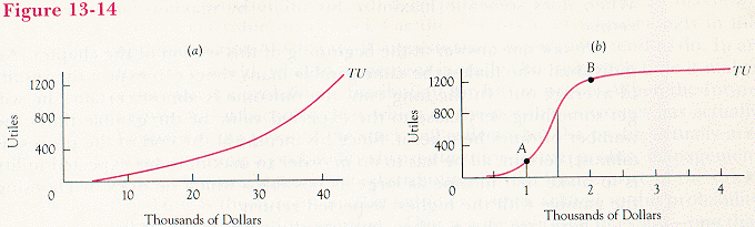
Total utility of income for a risk preferrer and for someone who is risk preferring for some incomes and risk averse for others. Figure 13-14b shows total utility of income for someone who requires about $1,500 to stay alive. Below that point, the marginal utility of income (the slope of total utility) increases with increasing income; above that point, it decreases.
We saw one answer at the beginning of this section of the chapter. An individual who makes the same gamble many times can expect the results to average out. In the long run, the outcome is almost certain--he will get something very close to the expected value of the gamble times the number of times he takes it. Since his income at the end of the process is (almost) certain, all he has to do in order to maximize his expected utility is to make that income as large as possible--which he does by choosing the gamble with the highest expected return.
There are three other important situations in which maximizing expected utility turns out to be equivalent to maximizing expected return. One is when the individual is risk-neutral, as shown on Figure 13-12. A second is when the size of the prospective gains and losses is small compared to one's income. If we consider only small changes in income, we can treat the marginal utility of income as constant; if the marginal utility of income is constant, then changes in utility are simply proportional to changes in income, so whatever choice maximizes expected return also maximizes expected utility.
One can see the same thing geometrically. Figure 13-15 is a magnified version of part of Figure 13-13a. If we consider only a very small range of income--between $19,900 and $20,000, for instance--the utility function is almost straight. For a straight-line utility function, as I showed earlier, maximizing expected utility is equivalent to maximizing expected return. So if we are considering only small changes in income, we should act as if we were risk neutral.
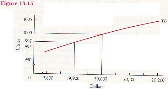
Magnified version of part of Figure 13-13a. Although the total utility curve shown on Figure 13-13a is curved, corresponding to risk aversion, any small section of it appears almost straight. This corresponds to the fact that the marginal utility of income is almost constant over small ranges of income; individuals are almost risk neutral for small gambles.
Next consider the case of a corporation that is trying to maximize the market value of its stock--as the discussion of takeover bids in the optional section of Chapter 9 suggests that corporations tend to do. In an uncertain world, what management is really choosing each time it makes a decision is a probability distribution for future profits. When the future arrives and it becomes clear which of the possible outcomes has actually happened, the price of the stock will reflect what the profits actually are. So in choosing a probability distribution for future profits, management is also choosing a probability distribution for the future price of the stock.
How is the current market value of a stock related to the probability distribution of its future value? That is a complicated question--one that occupies a good deal of the theory of financial markets; if you are an economics major, you will probably encounter it again. The short, but not entirely correct, answer is that the current price of the stock is the expected value of the future price--the average over all possible futures weighted by the probability of each. The reason is that the buyer of stock is in the same position as the gambler discussed earlier; he can average out his risks by buying a little stock in each of a large number of companies. If he does, his actual return will be very close to his expected return. If the price of any particular stock were significantly lower than the expected value of its future price, investors would all want to buy some of it; if the price were higher than the expected value of its future price, they would all want to sell some. The resulting market pressures force the current price toward the expected value of future prices.
If, as suggested above, management wishes to maximize the present price of its stock, it must try to maximize the expected value of its future price. It does that by maximizing the expected value of future profits. So it acts like the gambler we started with; it maximizes expected returns.
This is true only if the firm is trying to maximize the value of its stock. The threat of takeover bids has some tendency to make it do so. It is not clear how strong that tendency is--how closely that threat constrains management. To the extent that management succeeds in pursuing its own goals rather than those of the stockholders, the conclusion no longer holds. If the firm takes a risk and goes bankrupt, the (present and future) income of the chief executive may fall dramatically. If so, he may well be unwilling to make a decision that has a 50 percent chance of leading to bankruptcy even if it also has a 50 percent chance of tripling the firm's value.
Insurance. The existence of individuals who are risk averse provides one explanation for the existence of insurance. Suppose you have the utility function shown in Figure 13-13a. Your income is $20,000, but there is a small probability --0.01--of some accident that would reduce it to $10,000. The insurance company offers to insure you against that accident for a price of $100. Whether or not the accident happens, you give them $100. If the accident happens, they give you back $10,000. You now have a choice between two gambles--buying or not buying insurance. If you buy the insurance, then, whether or not the accident occurs, the outcome is the same--you have $20,000 minus the $100 you paid for the insurance (I assume the accident only affects your income). So for the first gamble, you have:
p1 = 1; R1 = $19,900; <U> = p1 x U(R1) = 997 utiles.
If you do not buy the insurance, you have:
p1 = 0.99; R1 = $20,000; U(R1) = 1,000 utiles;
p2 = 0.01; R2 = $10,000; U(R2) = 600 utiles;
<U> = [p1 x U(R1)] + [p2 x U(R2)] = 990 utiles + 6 utiles = 996 utiles.
You are better off with the insurance than without it, so you buy the insurance.
In the example as given, the expected return--measured in dollars--from buying the insurance was the same as the expected return from not buying it. Buying insurance was a fair gamble--you paid $100 in exchange for one chance in a hundred of receiving $10,000. The insurance company makes hundreds of thousands of such bets, so it will end up receiving, on average, almost exactly the expected return. If insurance is a fair gamble, the money coming in to buy insurance exactly balances the money going out to pay claims. The insurance company neither makes nor loses money; the client breaks even in money but gains in utility.
Insurance companies in the real world have expenses other than paying out claims--rent on their offices, commissions to their salespeople, and salaries for their administrators, claim investigators, adjusters, and lawyers. In order for an insurance company to cover all its expenses, the gamble it offers must be somewhat better than a fair one from its standpoint. If so, it is somewhat worse than fair from the standpoint of the company's clients.
The clients may still find that it is in their interest to accept the gamble and buy the insurance. If they are sufficiently risk averse, an insurance contract that lowers their expected return may still increase their expected utility. In the case discussed above, for example, it would still be worth buying the insurance even if the company charged $130 for it. It would not be worth buying at $140. You should be able to check those results for yourself by redoing the calculations that showed that the insurance was worth buying at $100.
Earlier I pointed out that with regard to risks that involve only small changes in income, everyone is (almost) risk neutral. One implication of this is that it is only worth insuring against large losses. Insurance is worse than a fair gamble from the standpoint of the customer, since the insurance company has to make enough to cover its expenses. For small losses, the difference between the marginal utility of income before and after the loss is not large enough to convert a loss in expected return into a gain in expected utility.
The Lottery-Insurance Puzzle. Buying a ticket in a lottery is the opposite of buying insurance. When you buy insurance, you accept an unfair gamble--a gamble that results, on average, in your having less money than if you had not accepted it--in order to reduce uncertainty. When you buy a lottery ticket, you also accept an unfair gamble--on average, the lottery pays out in prizes less than it takes in--but this time you do it in order to increase your uncertainty. If you are risk averse, it may make sense for you to buy insurance--but you should never buy lottery tickets. If you are a risk preferrer it may make sense for you to buy a lottery ticket--but you should never buy insurance.
This brings us to a puzzle that has bothered economists for at least 200 years--the lottery-insurance paradox. In the real world, the same people sometimes buy both insurance and lottery tickets. Some people both gamble when they know the odds are against them and buy insurance when they know the odds are against them. Can this be consistent with rational behavior?
There are at least two possible ways in which it can. One is illustrated on Figure 13-16. The individual with the utility function shown there is risk averse for one range of incomes and risk preferring for another, higher, range. If he starts at point A, in between the two regions, he may be interested in buying both insurance and lottery tickets. Insurance protects him against risks that move his income below A--where he is risk averse. Lottery tickets offer him the possibility (if he wins) of an income above A--where he is risk preferring.
This solution is logically possible, but it does not seem very plausible. Why should people have such peculiarly shaped utility functions, with the value to them of an additional dollar first falling with increasing income then rising again? And if they do, why should their incomes just happen to be near the border between the two regions?
Another explanation of the paradox is that in the real-world situation we observe, one of the conditions for our analysis does not hold. So far, we have been considering situations where the only important difference among the outcomes is money; the utility of each outcome depends only on the amount of money it leaves you with. It is not clear that this is true for the individuals who actually buy lottery tickets.
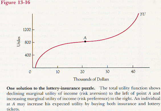
One solution to the lottery-insurance puzzle. The total utility function shows declining marginal utility of income (risk aversion) to the left of point A and increasing marginal utility of income (risk preference) to the right. An individual at A may increase his expected utility by buying both insurance and lottery tickets.
Consider the lotteries you have yourself been offered--by Reader's Digest, Publisher's Clearinghouse, and similar enterprises. The price is the price of a stamp, the payoff--lavishly illustrated with glossy photographs--a (very small) chance of a new Cadillac, a Caribbean vacation, an income of $20,000 a year for life. My rough calculations--based on a guess of how many people respond to the lottery--suggest that the value of the prize multiplied by the chance of getting it comes to less than the cost of the stamp. The expected return is negative.
Why then do so many people enter? The explanation I find most plausible is that what they are getting for their stamp is not merely one chance in a million of a $40,000 car. They are also getting a certainty of being able to daydream about getting the car--or the vacation or the income--from the time they send in the envelope until the winners are announced. The daydream is made more satisfying by the knowledge that there is a chance, even if a slim one, that they will actually win the prize. The lottery is not only selling a gamble. It is also selling a dream--and at a very low price.
This explanation has the disadvantage of pushing such lotteries out of the area where economics can say much about them; we know a good deal about rational gambling but very little about the market for dreams. It has the advantage of explaining not only the existence of lotteries but some of their characteristics. If lotteries exist to provide people a chance of money, why do the prizes often take other forms; why not give the winner $40,000 and let him decide whether to buy a Cadillac with it? That would not only improve the prize from the standpoint of the winner but would also save the sponsors the cost of all those glossy photographs of the prizes.
But many people may find it easier to daydream about their winnings if the winnings take a concrete form. So the sponsors (sometimes) make the prizes goods instead of money--and provide a wide variety of prizes to suit different tastes in daydreams. This seems to be especially true of "free" lotteries--ones where the price is a stamp and the sponsor pays for the prizes out of someone's advertising budget instead of out of ticket receipts. Lotteries that sell tickets seem more inclined to pay off in money--why I do not know.
In Chapter 1, I included in my definition of economics the assumption that individuals have reasonably simple objectives. You will have to decide for yourself whether a taste for daydreams is consistent with that assumption. If not, then we may have finally found something that is not an economic question--as demonstrated by our inability to use economics to answer it.
Near the beginning of this section, I said that John Von Neumann was responsible for combining the ideas of utility and choice under uncertainty. So far, I have shown how the two ideas are combined but have said very little about exactly what Von Neumann (in conjunction with economist Oskar Morgenstern) contributed. You may reasonably have concluded that the great idea was simply to assert "People maximize expected utility" and keep talking--in the hope that nobody would ask "Why?"
What Von Neumann and Morgenstern actually did was both more difficult and more subtle than that. They proved that if you assume that individual choice under uncertainty meets a few simple consistency conditions, it is always possible to assign utilities to outcomes in such a way that the decisions people actually make are the ones they would make if they were maximizing expected utility.
Von Neumann and Morgenstern start by considering an individual choosing among "lotteries." A lottery is a collection of outcomes, each with a probability. Some outcome must occur, so all the probabilities together add up to one. Just as, in considering ordinary utility functions, we assume that the individual can choose between any two bundles, so they assumed that given any two lotteries L and M, the individual either prefers L to M, prefers M to L, or is indifferent between them. They further assumed that preferences are transitive; if you prefer L to M and M to N, you must prefer L to N.
Another assumption was that in considering lotteries whose payoffs are themselves lotteries--probabilistic situations whose outcomes are themselves probabilistic situations--people combine probabilities in a mathematically correct fashion. If someone is offered a ticket giving him a 50 percent chance of winning a lottery ticket, which in turn gives him a 50 percent chance of winning a prize, he regards that compound lottery as equivalent to a ticket giving a 25 percent chance of winning the same prize--and similarly for any other combination of probabilities.
The remaining two assumptions involve the continuity of preferences. One is that if I prefer outcome A to outcome B, I also prefer to B any lottery that gives me some probability of getting A and guarantees that if I do not get A, I will get B. The final assumption is that if I prefer outcome A to outcome B and outcome B to outcome C, then there is some probability mix of A and C--some lottery containing only those outcomes--that I consider equivalent to B. To put it in different words, this says that as I move from a certainty of A to a certainty of C via various mixtures of the two, my utility changes continuously from U(A) to U(C). Since by assumption U(A) > U(B) > U(C)--that is what the "if" clause at the beginning of this paragraph says--as my utility moves continuously from U(A) to U(C) it must at some intermediate point be equal to U(B).
All of these assumptions seem reasonable as part of a description of "rational" or "consistent" behavior under uncertainty. If an individual's behavior satisfies them, it is possible to define a Von Neumann utility function--a utility for every outcome--such that the choices he actually makes are the choices he would make if he were trying to maximize his expected utility. That is what Von Neumann and Morgenstern proved.
In the optional section of Chapter 3, I pointed out that utility as then defined contained a considerable element of arbitrariness; utility functions were supposed to describe behavior, but exactly the same behavior could be described by many different utility functions. We could deduce from observing individuals' choices that they preferred A to B, but not by how much. Even the principle of declining marginal utility, to which I several times referred, is, strictly speaking, meaningless in that context; if you cannot measure the amount by which I prefer one alternative to another, then you cannot say whether the additional utility that I get when my income increases from $9,000/year to $10,000 is more or less than when it increases from $10,000 to $11,000. Declining marginal utility then has content only in the form of the declining marginal rate of substitution--a concept that, as I pointed out at the time, is closely related but not equivalent.
Once we accept the Von Neumann-Morgenstern definition of utility under uncertainty, that problem vanishes. The statement "I prefer outcome C to outcome B by twice as much as I prefer B to A" is equivalent to "I am indifferent between a certainty of B and a lottery that gives me a two-thirds chance of A and a one-third chance of C."
To see that the two statements are equivalent, we will work out the expected utilities for the two alternatives described in the second statement and show that the first statement implies that they are equal, as follows:
Let Lottery 1 consist of a certainty of B, Lottery 2 of a two-thirds chance of A and a one-third chance of C. We have for Lottery 1:
p1 = 1; U1 = U(B); <U> = U(B).
We have for Lottery 2:
p1 = 2/3; U1 = U(A);
p2 = 1/3; U2 = U(C);
<U> = p1U1 + p2U2 = 2/3 U(A) + 1/3 U(C).
Statement 1 tells us that:
U(C) - U(B) = 2 x (U(B) - U(A)).
Rearranging this gives us:
U(C) + 2 x U(A) = 3 x U(B);
2/3 U(A) + 1/3 U(C) = U(B). (Equation 5)
The left-hand side of Equation 5 is the expected utility of Lottery 2, and the right-hand side is the expected utility of Lottery 1, so the expected utilities of the two alternatives are the same; the individual is indifferent between them.
We have now shown that Statement 1 implies Statement 2. We could equally well have started with Statement 2 and worked backward to Statement 1. If each statement implies the other, then they are equivalent.
So using utility functions to describe choice among probabilistic alternatives makes the functions themselves considerably less arbitrary. In our earlier discussion of utility, the only meaningful statements were of the form "A has more utility to me than B" or, equivalently, "I prefer A to B." Now the statement "Going from A to B increases my utility by twice as much as going from C to D" (or, equivalently, "I prefer A to B twice as much as I prefer C to D") has meaning as well. If we can make quantitative comparisons of utility differences, we can also make quantitative comparisons of marginal utilities, so the principle of declining marginal utility means something. We saw exactly what it meant a few pages ago; the statement "My marginal utility for income is declining" is equivalent to "I am risk averse." Similarly, the statement "My marginal utility for ice cream cones is declining" is equivalent to "I am risk averse if expected return is in ice cream cones rather than in dollars. I would not accept a gamble that consisted of a 50 percent chance of getting an ice cream cone and a 50 percent chance of losing one."
We have eliminated much of the arbitrariness from utility functions but not all of it. Nothing we have done tells us how big a utile is, so a change in scale is still possible. If I say that I prefer A to B by 10 utiles, B to C by 5, and C to D by 2, while you insist that the correct numbers are 20, 10, and 4, no possible observation of my behavior could prove one of us right and one wrong. We agree about the order of preferences; we agree about their relative intensity--all we disagree about is the size of the unit in which we are measuring them.
It is also true that nothing we have done tells us where the zero of the utility function is. If I claim that my utilities for outcomes A, B, and C are 0, 10, 30, while you claim they are - 10, 0, and 20, there is again no way of settling the disagreement. We agree about the order, we agree about the differences--all we disagree about is which alternative has zero utility. So changes in the utility function that consist of adding the same amount to all utilities (changing the zero), or multiplying all utilities by the same number (changing the scale), or both, do not really change the utility function. The numbers are different, but the behavior described is exactly the same. This means, for those of you who happen to be mathematicians, that utility functions are arbitrary with respect to linear transformations.
My own preference is to define zero as nonexistence or death; that, after all, is the one outcome in which one gets, so far as I know, neither pleasure nor pain. A friend and colleague once commented to me that she was not certain whether the present value of utility at birth was positive or negative--meaning that she was not sure whether, on net, life was worth living. I concluded that her life had been much harder than mine.
You have decided to buy a car and are choosing between two alternatives: a Honda Accord and a Nissan Stanza. From previous experience, you expect that you will like one of the cars better than the other, but unfortunately you do not know which. If forced to state your opinions more precisely, you would say that you think your consumer surplus would be $500 higher if you bought the better car, and the probability that the Accord is better than the Stanza is exactly 0.5 .
You consider two strategies. You can randomly choose one of the cars and buy it. Alternatively, you can rent an Accord for your next long trip, a Stanza for the trip after that, and then decide which to buy. You believe that after having driven each car a substantial distance, you will know with certainty which you like better. Since it is more expensive to rent a car than to use a car you own, the second strategy will cost you an extra $200. Should you do it?
The answer depends on your utility function. You are choosing between two lotteries. The first has payoffs of $0 and $500, each with probability 0.5. The second has a certain payoff of $300, since you get the extra consumer surplus but pay $200 for it. If you are risk neutral or risk averse, you prefer a certainty of $300 to a 0.5 chance of $500, so you rent the cars before you buy. If you are a strong risk preferrer, you prefer the gamble, so you buy without renting.
This simple problem illustrates the general idea of buying information. By paying some search cost you can reduce uncertainty, improving, on average, the outcomes of your decisions. To decide whether the search cost is worth paying, you compare expected utility without search to expected utility with search, remembering to include the cost of the search in your calculation.
In this particular case you had only two alternatives, to search or not to search, and searching gave you complete information--you knew with certainty which car you preferred. In more general cases you may have to decide just how much searching to do; the more you search, the better your information. The correct rule is to search up to the point where the value of the marginal increase in your expected utility from searching a little more is just equal to the cost.
One example of such behavior that has received a great deal of attention is the problem of job search. Many people who consider themselves unemployed could find a job almost instantly--if they were willing to wait on tables, or wash dishes, or drive a cab. What they are looking for is not a job but a good job. The longer they look, the better, on average, will be the best job opportunity they find. Their rational strategy is to keep looking as long as they expect to gain more from additional search than it costs them. Such search unemployment makes up a significant fraction of the measured unemployment rate.
One implication of this is that increases in unemployment compensation tend to increase the unemployment rate. The reason is not that the unemployed are lazy bums who prefer collecting unemployment to working, but that they are rational searchers. The higher the level of unemployment compensation is, the lower the cost of being unemployed while searching for a job. The less it costs to search, the more searching it pays to do.
Issues associated with acquiring and using information provide some of the most interesting and difficult questions in economics. They first appeared back in Chapter 1, where I briefly mentioned the problem of incorporating information costs into the definition of rationality, and will reappear in Chapter 18.
In the first 11 chapters of this book, we used economics to understand how markets work in a certain and unchanging world. It may have occurred to you that doing so was a waste of time, since we live in a world that is uncertain and changing.
Looking back at what we have done in Chapters 12 and 13, you may now see why the book is organized in this way. In Chapter 12, we learned how to analyze choice in a changing (but certain) world using the same tools developed for an unchanging world--simply evaluate costs and benefits in terms of present values instead of annual flows. Now we have learned how to analyze choice in an uncertain world by again using the same tools; we merely evaluate costs and benefits by comparing the expected utilities of probabilistic outcomes instead of the utilities of certain outcomes. Combining the lessons of the two chapters in order to analyze choice in a world that is both changing and uncertain would be straightforward--evaluate choices in terms of the present value of expected utility.
What we have done is to first solve economics in a simple world and then show that the more complicated and realistic world can, for purposes of economic analysis, be reduced to the simple one. Introducing time and change does create some new problems, such as those associated with sunk costs. Yet it is still true that in learning to deal with the simple world of Chapters 1-11 we learned most of the basic ideas of economics, and that in Chapters 12 and 13 we have taken a large step towards making those ideas applicable to the world we live in.
The concept of utility originated during the nineteenth century among thinkers interested in both philosophy and economics. It was proposed as an answer to the question "What should a society maximize?" The utilitarians asserted that a society should be designed to maximize the total utility of its members.
Their position has been heavily criticized over the years and is now in poor repute among philosophers. One of the major criticisms was that although we can, in principle, determine whether you prefer A to B by more than you prefer C to D, there seems to be no way of determining whether I prefer A to B by more than you prefer C to D. There is no way of making interpersonal comparisons of utility, no way of deciding whether a change that benefits me (gives me A instead of B) and injures you (gives you D instead of C) increases or decreases total utility.
One possible reply to this criticism of utilitarianism goes as follows. Suppose we define utility in the sense of Von Neumann and Morgenstern and use it to evaluate some question such as "Should the United States abolish all tariffs?" It turns out that the utilitarian rule--"Maximize total utility"--is equivalent to another rule that some find intuitively more persuasive: "Choose that alternative you would prefer if you knew you were going to be one of the people affected but had no idea which."
Why are the two equivalent? If I have no idea who I am going to be, I presumably have an equal probability p of being each person; if there are N people involved, then p = 1/N. If we write the utility of person i as Ui, then the lottery that consists of a probability p of being each person has an expected utility:
<U> = ![]() piUi =
piUi = ![]() pUi, = p
pUi, = p ![]() Ui.
Ui.
But ![]() Ui is simply the total utility of the society, so
whichever alternative maximizes total utility also maximizes
<U>.
Ui is simply the total utility of the society, so
whichever alternative maximizes total utility also maximizes
<U>.
PROBLEMS
1. How should the developers of a new airliner take account of the plane's design costs in deciding whether to design and build the plane? In determining the price to charge airline companies? Should they suspend production if they find that they cannot obtain a price that will cover design costs?
2. After reading this chapter, you are considering dropping this course. What costs should you take into account in deciding whether to do so? What costs that you should ignore in that decision should you have taken into account in deciding to take the course in the first place?
3. Figure 13-17a shows the cost curves for producing typewriters in a typewriter factory. The inputs are available in perfectly elastic supply; all firms are identical and there are no restrictions on starting new firms. Each firm can run one factory.
a. Draw the supply curve for one firm; label it Sf. Draw the supply curve for the industry, label it Si. Da is the demand curve for typewriters; everyone expects it to stay the same for ever. How many are sold at what price? How many firms are there?
b.The demand curve shifts up to Db. It takes a year to build a new typewriter factory. Draw the short run supply curve SSR, showing price as a function of quantity over times too short to build more factories. A month after the change, how many typewriters are sold at what price?
c. AC on Figure 13-17a includes the cost of building a typewriter factory, which is three million dollars. Factories last for 10 years; the interest rate is zero and factories have no scrap value. After the firms have adjusted to Db, the word processor is invented and the demand curve for typewriters suddently shifts down to Dc. Everyone expects it to remain there forever. Immediately after the change, what is the price of a typewriter?
d. The demand curve remains at Dc. Fifty years later, what is the price of a typewriter? How many are produced each year?
4. Long-run total cost includes both short-run and long-run expenses, so for any quantity long-run total cost must be larger than short-run total cost. True or False? Discuss.
The following problems refer to the optional section:
5. You have $30,000; your utility function is shown by Figure 13-12. There is one chance in a hundred that your house will be struck by lightning, in which case it will cost $10,000 to repair it. What is the highest price you would be willing to pay, if necessary, for a lightning rod to protect your house?
6. Answer Problem 6 for the utility function of Figure 13-13a.
7. Figure 13-18 is identical to Figure 13-13a, with the addition of a line connecting two points--A and E--on the utility function. I claim that point C, halfway between points A and E, represents the utility (vertical axis) and expected return (horizontal axis) of a fifty-fifty gamble between A ($10,000) and E ($30,000); the fact that C is below the graph of the utility function indicates that you prefer a certainty with the same expected return ($20,000) to such a gamble. Similarly, I claim that point B represents a gamble with a 75 percent chance of giving you A and a 25 percent chance of giving you E, and that point D represents a gamble with a 25 percent chance of A and a 75 percent chance of E.
Prove that these claims are true--that the vertical position of each point equals the expected utility of the corresponding gamble and that the horizontal position equals the expected return.
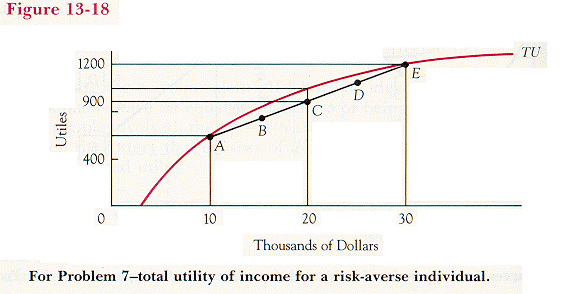
8. In the text, I asserted that declining marginal utility of income was equivalent to risk aversion and that increasing marginal utility of income was equivalent to risk preference. While I gave examples, I did not prove that the assertion was true in general. Use the result of Problem 10 to do so.
9. In discussing risk aversion, I have only considered alternatives that are measured in money. Suppose you are gambling in apples instead. Is it possible for someone to be a risk preferrer in terms of dollars and a risk averter in terms of apples? Vice versa? Does it depend on whether there is a market on which you can buy and sell apples?
10. In one episode of Star Trek, Spock is in an orbiting landing craft that is running out of fuel and will shortly crash. Captain Kirk and the Enterprise are about to leave the planet, having somehow misplaced one landing craft and science officer. Spock fires his rockets, burning up all the remaining fuel, in the hope that the Enterprise will notice the flare and come rescue him. Later Kirk twits the supremely logical Spock with irrationality, for having traded his last few hours of fuel for a one in a hundred chance of rescue. Is Kirk correct? Was Spock's behavior irrational?
The original discussion of Von Neumann utility is in John Von Neumann and Oskar Morgenstern, Theory of Games and Economic Behavior (Princeton: Princeton University Press, 1944), Chapter 1.
A classic discussion of the lottery-insurance paradox is Milton Friedman and Leonard J. Savage, "The Utility Analysis of Choices Involving Risk," Journal of Political Economy, Vol. 56, No. 4 (August, 1948), pp. 279-304.
For discussions of some of the philosophical issues associated with what, if anything, the good society would maximize, you may wish to look at two important books: Robert Nozick, Anarchy, State and Utopia (New York: Basic Books, Inc., 1974) and John Rawls, A Theory of Justice (Cambridge: Harvard University Press, 1971). You may also be interested in an essay of mine on the question of what you should maximize if one of the variables is the number of people; in that situation maximizing total utility and maximizing average utility lead to different results. It is:
"What Does Optimum Population Mean," Research in Population Economics, Vol. III (1981), Eds. Simon and Lindert.
Next