Three questions that are often asked of economists are: What is the distribution of income? What determines the distribution of income? Is it fair? In this part of the chapter, I will have a little to say about the first question and a good deal to say about the second. Whether what I say has anything to do with the third, you will have to decide for yourself.

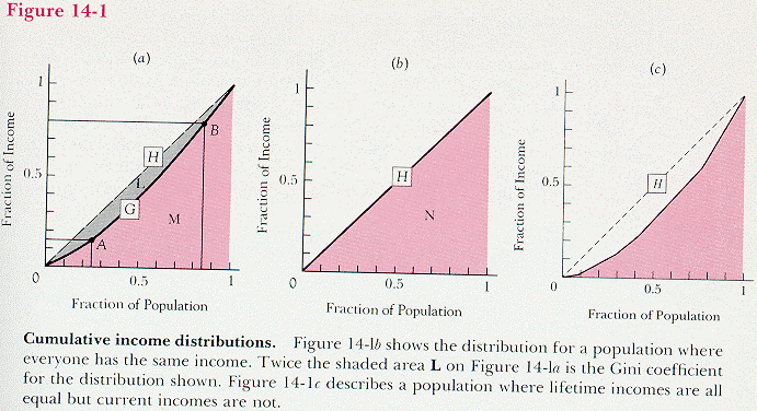
Curve G on Figure 14-1a is a graph of the cumulative income distribution for some imaginary society. The horizontal axis shows a fraction of the population, ranked by income; the vertical axis shows what fraction of national income goes to that part of the population. Point A on the figure shows that the bottom 25 percent of the population receives about 15 percent of national income; point B shows that the bottom 85 percent of the population receives about 80 percent of national income.

Curve H on Figure 14-lb is a similar graph for a society in which everyone has the same income. It is a straight line. Since everyone has the same income, the "bottom" 10 percent of the population has 10 percent of the income, the bottom 50 percent has 50 percent, and so on. Line G on Figure 14-la, which shows an unequal distribution, must lie below line H, since for an unequal distribution the bottom N percent of the population must have less than N percent of the income. Hence the colored area M in Figure 14-la must be less than the colored area N in Figure 14-1b; their difference is the shaded area L. To make this clearer, I have also shown H on Figure 14-1a.

Twice the area of L on Figure 14-la, called the Gini coefficient, is a simple measure of how unequal the income distribution of Figure 14-la is. Since the graph is a 1x1 square, its entire area, equal to twice the triangle N on Figure 14-1b, is simply 1. So the Gini coefficient can also be defined as the ratio of area L to area N, or as the ratio of L to L+M. The closer that ratio is to zero, the more nearly equal the income distribution. Various estimates of what the Gini coefficient is for the United States at present and how it has varied over time have been made.

One problem with most such estimates is that they measure current income rather than lifetime income. To see why this is a problem, imagine that we have a society in which everyone follows an identical career pattern. From ages 18 to 22 everyone is a student, earning $5,000/year at various part-time jobs. From 23 to 30 everyone has a job with a salary of $20,000/year. From 31 to 50 everyone makes $30,000/year; from 51 to 65 everyone makes $40,000/year and then retires on a pension of $15,000/year and lives to 77. Figure 14-1c shows the resulting income distribution, seen at a single instant. If you calculate a Gini coefficient from the figure, it is about .23.

This is a perfectly egalitarian society, since everyone's income follows the same pattern; but the income distribution appears far from equal on the graph, and the Gini coefficient is not equal to zero, as it should be if all incomes are equal. The reason is that, at any one instant, some people are students, some are employees with varying degrees of experience, and some are retired. So if you look at a cross section of the society at a single instant, incomes appear quite unequal. Both the cumulative income distribution shown on Figure 14-1c and the corresponding Gini coefficient are the same as for a society where one twelfth of the people have an income of $5,000/year, two tenths have $15,000/year, and so on--with everyone having the same income for his whole lifetime. The Gini coefficient as usually calculated tells us how unequal incomes are at one instant in time but does not distinguish between inequality due to different people being in different stages of their earning cycle and inequality due to some people being richer or more talented than others.

---

---

Most estimates of the income distribution are done in this way, which suggests that most estimates considerably overstate actual inequality. One study I saw that tried to allow for such effects concluded that they roughly doubled the measured Gini coefficient. If that result is correct, then if you consider lifetime income rather than income at one instant in time, the United States income distribution is about half as unequal as conventional estimates suggest.

A similar problem arises when one tries to figure out whether some particular program, such as social security, redistributes from the rich to the poor or from the poor to the rich. To see how the problem arises, we will start by considering a social security program that has no redistributional effect at all; everyone gets back just what he paid in, plus accumulated interest. (This is not the way the real social security system works.) Since payments are made when you are employed and benefits received when you are retired, payments are made by someone with a higher income than the person who receives the benefits--not because the money is going from rich to poor but because it is going from you when you have a higher income to you in a later year when you have a lower income. If you look at a cross section of the population, it appears that social security redistributes from rich to poor--the people who are paying are richer than those receiving--even though, in this case, there is no redistribution at all.

It is not clear what the distributional effect of the real social security system is; it may actually redistribute from lower to higher income workers. The higher income worker typically starts working--and paying in--at an older age, which reduces his total payments, and lives longer, which increases his total benefits. Whether these effects are outweighed by other features of the system that provide relative advantages to the poor is not clear. What is clear is that a comparison of the incomes of those who in any particular year are receiving social security to the incomes of those who are paying for it always shows the system transferring income from richer to poorer--and that result tells us almost nothing about the real effect of the system on the distribution of income.

A third problem arises when we try to measure changes in the distribution of income over time. To do so, we require statistics on what incomes are and were. The obvious source for such statistics is the Internal Revenue Service (IRS). But IRS statistics tell us not what people earned but what they reported. Over the past 70 years, the rate at which income is taxed has increased enormously. The higher the tax rate, the higher the incentive for people with high incomes to make them appear lower than they are, at least when the IRS is looking. So IRS figures almost certainly underestimate how well the rich are doing in recent decades as compared to the earlier part of the century. The recent tax reform act substantially lowered the tax rate on the highest brackets; it will be interesting to see if one result is an increase in the number of people who confess to having high incomes, and thus in (measured) income inequality.

The conclusion from all of this is that statements about the income distribution, about how it has changed over time and about how it is changed by particular government programs, should be viewed with considerable skepticism.

You are a worker. What determines your salary? One answer is "the most you are worth to any employer." Another is "the least you are willing to work for." Both are true--for exactly the same reason that the price of a good is equal both to its value to the consumer and to its cost of production.

To Each According to His Product. Consider the president of a pants company, trying to decide how many workers to hire. Holding all other inputs constant, he calculates how many extra pairs of pants the firm produces for each extra worker hired; the answer is five pairs per day. Five pairs of pants per day is the marginal physical product of a worker, as explained in Chapter 9.

Suppose a pair of pants sells for $10. The marginal revenue product of a worker is then $50/day. If an employer hires one more worker, output rises by five pairs of pants per day, the firm sells them for $10/pair, so revenue increases by $50/ day. Since marginal product is defined with all other inputs held constant, cost rises by what the firm has to pay the extra worker. As long as the cost of hiring another worker is less than $50/day, the firm increases its profit by hiring him. As it hires more workers, their marginal product drops, because of the law of diminishing returns. The firm stops hiring when marginal revenue product equals the wage it must pay to get more workers. So a worker's wage equals what he produces--the value of the extra production from adding one more worker while keeping all other inputs fixed. If we consider a range of different wages, this implies, as we saw back in Chapter 9, that the firm's demand curve for an input is simply that input's marginal revenue product curve.

The logic of the situation is the same that gave us demand curves from marginal value curves and supply curves from marginal cost curves. It applies not only to workers but to all inputs--as was pointed out in Chapter 9. As long as the producer can buy as much of an input as he likes at some price--as long, in other words, as he is a price taker on the market for his inputs--he will buy it up to the point where its marginal revenue product equals its price. Hence the prices received by the owners of all inputs to production--the wages of labor, the rent of land, the interest on capital--are equal to the marginal revenue products of those inputs. Since income ultimately comes from selling inputs, this appears to be an explanation of the income distribution.

To Each According to His Cost. That each factor receives its marginal revenue product is a true statement about the income distribution (provided we are only considering price takers--there are additional complications for price searchers), but it is not an explanation of the income distribution. One way of seeing that is to note that it is also true that each factor gets its marginal cost of production. A worker who can choose how many hours he wants to work will work up to the point where his wage equals the marginal value of his leisure--the cost, to him, of working an additional hour. Hence his wage is equal to what it costs him to work. Just as we saw back in Chapter 5, the worker's supply curve for his own labor equals his marginal disvalue of labor (value of leisure) curve. Similarly, individuals will save (producing capital) up to the point at which the cost of giving up a little more present consumption in exchange for future consumption just balances what they gain by doing so--the interest rate. So the interest on capital is equal to the marginal cost of producing it.

One Explanation Too Many? We appear to have two explanations of the distribution of income--which some might consider one explanation too many. But neither is complete by itself. Labor receives its marginal product--but the marginal product of labor is determined in part by how much labor (and capital and land and . . .) is being used; the law of diminishing returns tells us that as we increase the amount of one input while holding the others constant, the marginal product of that input eventually starts to go down. Labor is paid its marginal cost of production--but that cost depends in part on how much labor is being sold; the law of declining marginal utility, applied to leisure, implies that the cost of working one more hour depends in part on how many hours you are working.

What we actually have is a description of equilibrium on the market for inputs--the same description we got some chapters earlier when we were considering the market for final goods. The full explanation of the income distribution is that the price of an input is equal to both its marginal cost of production and its marginal revenue product, and the quantity of the input sold and used is that quantity for which the marginal cost of production and the marginal revenue product are equal. (Marginal) cost equals price equals (marginal) value.

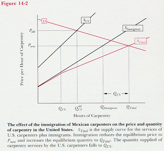
This conclusion is useful for seeing how various changes affect the distribution of income. Suppose the number of carpenters suddenly increases, due to the immigration of thousands of new carpenters from Mexico. Both before and after the change, carpenters receive their marginal revenue product. Both before and after, they receive a wage equal to the marginal value of the last hour of leisure they give up.

But the wage after the migration is lower than the wage before. Since the supply of carpenters is higher than before, the equilibrium wage is lower. At that lower wage more carpenters are hired and their marginal product is therefore lower. With lower wages, the existing carpenters work fewer hours (assuming a normally shaped supply curve for their labor) and, when they are working fewer hours, have more leisure and value the marginal hour of leisure less. Some carpenters--those with particularly good alternative occupations--find that, at the lower wage, they are better off doing something else. The marginal cost to the worker of working an additional hour falls, either because the marginal hour is worked by one of the old carpenters who is now working fewer hours or because the marginal carpenter is now one of the new immigrants.

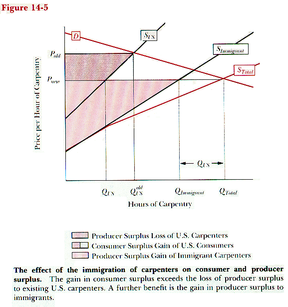
The change is shown on Figure 14-2. D is the demand curve for the services of carpenters ("carpentry") in the United States S_US is the supply curve for the services of U.S. carpenters before the new immigrants arrive; its intersection with D gives us the equilibrium price (P_old) and quantity(Q_US^old) for carpentry before the immigration. S_Immigrant is the supply curve of the new immigrants. S_Total is the total supply curve--the horizontal sum of S_US and S_Immigrant. Its intersection with D gives us the equilibrium price (P_new) and quantity (Q_Total) for carpentry after the immigration.

Looking at the figure, we observe that the wages of carpenters (the price of carpentry) have fallen. Some of the old carpenters have left the profession, some (Q_US) remain. Back in Chapter 5 we saw that the supply curve for labor is equal to the horizontal sum of the marginal cost curves of the laborers. So the marginal carpenter before the change valued his time at P_old and the marginal carpenter after the change valued it at P_new<P_old. In the case shown, Q_US>0; some U.S. carpenters remain in business, so marginal carpenters include both immigrants and U.S. carpenters willing to do some carpentry even at the lower wage.

Immigration is not the only thing that can affect the wage rate. Increases in the other factors of production will tend to increase the marginal product of labor, and hence its wage; decreases will have the opposite effect. Changes in technology can also alter the marginal product of labor or other inputs. If someone invents a computer program that does a better job than a human of teaching children basic skills, perhaps by converting reading, writing and arithmetic lessons into exciting video games, a substantial amount of human labor will have been replaced by capital. The demand for labor has decreased, the demand for capital has increased, so when equilibrium is reestablished wages will be a little lower than before the change and the return on capital, the interest rate, a little higher.

Once we know who owns inputs and how much each of the inputs gets, we also know the distribution of income. If I own 100 acres of land and land rents for $50/acre, I receive an income of $5,000/year from my land. If I also sell 2,000 hours per year of my own labor at $20/hour, I receive an income of $40,000/year from my labor. If these are the only inputs to production that I own, my total income is $45,000/year. We can in the same way calculate everyone else's income, giving us the distribution of income for the whole society.

One question often asked is, "Is this distribution just?" Supporters of the market system sometimes defend it by arguing that everyone gets what he produces, which seems fair. The wages of the laborer are equal to the market value of the additional output resulting from his labor, the interest received by the capitalist is equal to the value of the additional output resulting from the capital he has saved and invested, and so on. If the initial distribution of the ownership of inputs is just and if the principle "you are entitled to what you produce" is a legitimate one, it seems that the final distribution of income has been justified,

Even if you argue, as many would, that some inputs belong to the wrong people--for instance, that much of the land in the United States was unjustly stolen from the American Indians and should be given back--the argument still seems to justify a large part of the existing division of income. In a modern economy such as that of the United States at present, most income goes to human inputs--labor and the human capital embodied in learned skills--and most people would agree that a worker legitimately owns himself

Another way in which one might try to justify the present distribution of income is by appealing to the second half of the market equality--price equals cost of production. If the principle "to each according to what he has sacrificed in order to produce" is appealing to you, you can argue that the capitalist deserves the interest he receives because it represents the cost to him of postponing his consumption--giving up consumption now in exchange for more consumption later--and that the worker deserves his salary because it just makes up to him for the leisure he had to give up in order to work.

If you are completely satisfied by either of these arguments, you have probably not entirely understood them. The product and the cost that equal price are marginal product and marginal cost. The worker's salary just compensates him for the last hour he works--but he gets the same salary for all the hours he works. The interest collected by the capitalist equals the value of the additional production made possible by the addition of his capital--but the marginal revenue product of capital depends, in part, on how much labor, land, and other inputs are being used. Pure capital, all by itself, cannot produce much.

We are left with the problem of how to define a fair division of goods when the goods are produced not by any single person but by the combined efforts of many. While "payment according to marginal product" is a possible rule for division, and one that describes a large part of what actually happens in a market economy, it is far from clear whether it is a fair rule, or even what fairness means in such a context. Fortunately, determining what is fair is one of the (few?) problems that is not part of economics.

So far, we have used our analysis of the distribution of income to try to determine whether it is just. The same analysis can also be used to help us answer a question of considerable interest to many of us: How do I find out whether some particular economic change helps or hurts me? The answer, put simply, is that an increase in the supply of an input I own drives down its price (and marginal revenue product) and so decreases my income. The same is true for an increase in the supply of an input that is a close substitute for an input I own. If I happen to own an oil well, I will regard someone else's discovery of a new field of natural gas--or a process for producing power by thermonuclear fusion--as bad news.

An increase in the supply of an input used with the input I own (a complement in production) has the opposite effect. As the relative amount of my input used in production declines, its marginal product increases (the principle of diminishing returns, applied in reverse). If I own an oil well, I will be in favor of the construction of new highways.

Economic changes can affect what I buy as well as what I sell. Increases in the supply of goods I buy, or of inputs used to produce goods I buy, lower the price of those goods and so tend to benefit me. Decreases in their supply tend to make me worse off, for the same reason.

This may help answer the practical question of what things I ought to be for or against in some cases, but not in very many. It is clear enough that if I am a (selfish) physician, I should be in favor of restrictive licensing laws that keep down the number of physicians, and that if I am a (selfish) patient, I should be against them. It is much less clear how I should view the effect on my welfare of government deficits, restrictions on immigration, laws controlling the use of land, or any of a myriad of other things that do not directly affect the supply of the particular inputs I happen to own.

You may by now have realized that economics involves a continual balancing act between unrealistic simplification and unworkable complication. Chapter 8 was a prime example of the latter; the attempt to construct a complete description of even a simple economy involves a system of equations whose solution is well beyond the capacity of any existing computer.

In Part 2, I will swing us back in the other direction by showing how even a relatively complicated economy, such as the one we live in, can be viewed for some purposes as having only three inputs to production. This approach makes it possible to say something about how a particular person is affected by changes in the supply, demand, and price of goods that he neither buys nor sells.

Consider apples. For most purposes, we talk about the "supply of apples," the "price of apples," and so on. But, strictly speaking, a Golden Delicious apple, a Jonathan apple, and a Granny Smith apple are three different things. Even more strictly speaking, two Jonathan apples are different things; one is a little prettier, a little sweeter, or whatever. Even if we considered two identical apples, they would still be in different places, and the location of a good is one of its important characteristics; oil companies spend large sums converting crude petroleum two miles down into (identical) crude petroleum in a tank above ground.

For some purposes, it is convenient to make very fine distinctions, for others it is not; one cost of fine distinctions is that they make analysis more complicated. It is more precise to treat Golden Delicious apples and Red Delicious apples as two different goods that happen to be close substitutes; it is simpler to treat them as the same good.

Treating goods as close substitutes has almost the same effect as treating them as the same good. If they are the same good, an increase in the price of one implies an exactly equal increase in the price of the other, since they must sell for the same price. If they are substitutes, an increase in the price of one leads to an increase in the demand for the other, and hence an increase in its price. If they are sufficiently close substitutes--and if one unit of one good substitutes for one unit of the other--then an increase in the price of one produces an almost equal increase in the price of the other. To say that two things are both units of the same good is equivalent to saying that they are perfect substitutes for each other, as one piece of paper is a perfect substitute for another even though the two pieces are not literally identical--they would look slightly different under a microscope.

One could make a simple picture complicated by viewing each apple as a different good. I am instead going to make a complicated picture simple by viewing many different things as one good. This is how it works.

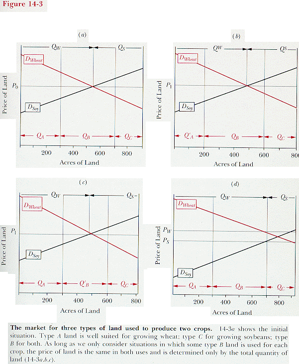
Consider three kinds of land--type A, type B, and type C. Suppose type A land is especially good for growing wheat, type C for growing soybeans, and type B good for both; for simplicity let an acre of A or B be equally good at producing wheat, and an acre of B or C equally good at producing soybeans. Further suppose supply and demand conditions are such that all the type A land is used for wheat, all the type C for soybeans, and some type B for each.

Under these circumstances, the prices of all three grades of land must be the same. The price of an acre of type A land is the present value of the net revenue (revenue minus production costs) of producing wheat on it; so is the price of an acre of type B land being used to produce wheat. Since types A and B land are equally good at producing wheat, the two prices must be the same. The price of an acre of type C land is the present value of the net revenue from producing soybeans on it--so is the price of an acre of type B land that is used for producing soybeans.

But all type B land must have the same price, whatever it is used for. If it did not, if, for instance, land used to produce soybeans was worth more than identical land used to produce wheat, then land would shift out of wheat production and into soybean production, driving the price of soybeans down and the price of wheat up. This process would continue until either the land was equally valuable in both uses or all of the type B land was used for soybeans.

Suppose a flood wipes out 100 acres of type A land. The initial effect is to raise the market price of wheat and of land growing wheat. Some type B land is now shifted from soybeans to the (more profitable) wheat. The quantity of wheat supplied increases, driving the price of wheat part of the way back down toward what it was before the flood. The quantity of soybeans supplied decreases, since some land that had been producing soybeans is now producing wheat; the price of soybeans rises. When equilibrium is reestablished, the prices of all three kinds of land are again the same. If they were not, more B land would shift from one crop to the other until they were. The final effect on the prices of wheat, soybeans, and land is the same as if the flood had wiped out 100 acres of type C land or of type B land.

Figures 14-3a, 14-3b, and 14-3c show the argument in graphical form; they illustrate the market for land used to grow wheat and soybeans. D_Wheat and D_Soy are the demand curves not for wheat and soybeans but for land used to grow them. The quantity of land used for wheat (Q_W) is measured from the left axis, the quantity used for soybeans (Q_S) from the right axis. Wheat land consists of all of the type A land (Q_A) plus part of the type B land; soybean land consists of the rest of the type B land plus all of the type C land (Q_C). The type B land is divided between wheat and soybeans in such a way as to make its price the same in either use.

Figure 14-3a shows the initial situation; the price of land in either use is P₀. Figure 14-3b shows the situation after a flood has eliminated 100 acres of type A land, reducing its total quantity to Q_A'=Q_A-100. Figure 14-3c shows what happens if the flood hits the type B land instead; quantity of type A land is back to Q_A, but quantity of type B land is now Q_B'=Q_B-100. You should be able to satisfy yourself that the price of land, P₁, is and must be the same on Figures 14-3b and c (and greater than the original price P₀), and the same for both uses of the land.

Figure 14-3d shows a situation where the prices of land used for wheat and land used for soybeans are no longer the same. The demand curves have shifted. There is no longer any way of dividing the type B land between the two uses that will make the price equal in both; even with all of it used to grow wheat, the price of wheat land (P_W) is still higher than the price of soybean land (P_S). No more land shifts from soybeans to wheat because the only land still being used to grow soybeans is type C land, which is badly suited for growing wheat.

As long as we only consider changes in supply and demand (of land, wheat, and soybeans) that leave some type B land growing soybeans and some growing wheat, as on 14-3a, b, c but not d, the situation is the same as if all the land were identical! We cannot directly replace type A land with type C land (or vice versa), but we can do so indirectly by replacing type A land with some type B land (converting it from soybeans to wheat) and replacing the type B land with type C land. The price of all three kinds of land is the same, and all we need to know is the total supply of land. In analyzing this particular economy, we can reduce three different inputs--types A, B, and C land--into one.

When the supply of land suited for one crop--say, corn--decreases, the price of that crop goes up. Land that, at the old price of corn, was used to grow some other crop that brought in a slightly higher income now generates more income by producing corn, so such land shifts out of other crops and into corn. By doing so, it transmits the decreased supply (and increased price) to the land used for what such marginal land was previously producing. A decrease in the supply of any one kind of land ultimately raises the price of all land, as does an increase in the demand for any one kind of land.

Land is not the only "good" that can be treated in this way. There are three traditional factors of production--land, labor, and capital. Each is really a group of goods that substitute for each other sufficiently well to be treated, for many purposes, as a single good. In each case, what is essential is not that every unit can directly substitute for every other unit, but that there are always some marginal units that can shift from one use to another so as to transmit changes affecting one good in the group to all the others.

Most of the inputs to production can be classified as either land, labor, or capital, although not always in the way a noneconomist might expect--a surgeon, for example, is largely capital! So this approach allows us to view even a very complicated economy as if it had only three inputs to production. For analyzing short-run changes, the approach is not very useful--an increased demand for economists is unlikely to have much immediate effect on either the wages of ditchdiggers or the interest on bonds, although economists are a mixture of labor and capital, the wages of ditchdiggers are a measure of the price of labor, and the interest on bonds is a measure of the price of capital.

In the longer run, it is easier to transform one form of labor or capital into another. If the demand for economists increases, then more people will become economists--instead of ditchdiggers or political scientists or secretaries. Training additional economists will require that people--the economics students themselves, their parents, investors lending them money for their education, or the government--spend money now for a return in the future. So less money will be available to be spent now for a future return in other ways--to build factories, do research, or train people in other professions. Labor and capital are being shifted into producing economics and out of producing ditches, cars, and many other things.

In the short run, the economy is less flexible than in the long run, as has been pointed out before. In the short run, the only people who can do economics are economists; the only ways to produce more economics are by getting some economists presently producing economics to produce more of it, or by getting economists who are presently doing other things--writing textbooks, for example, or loafing on the French Riviera--to go back to doing economics. In the long run, the factors of production can be used to produce more economists, hence more economics--and similarly with anything else. So the factors of production are more useful for understanding what happens in the long term than for understanding what happens in the short term.

In the next few sections of the book, I will discuss the three traditional factors of production--labor, land, and capital--so that you can see what they are and how they differ from each other.

Workers combine in themselves two different factors of production--raw labor and human capital. To produce a steelworker, one requires both a person and training; the latter, like any other investment, involves consuming inputs now in exchange for future returns, so it is properly classified as a form of capital. The wages of a worker can then be divided into the return on raw labor and the return on the laborer's human capital.

People are not all identical; even before training, a 6-foot man can probably dig more ditches per day than a 5-foot woman. To some extent, one can deal with this by thinking of different people as containing different amounts of raw labor. The situation would be simple if the person who could dig twice as many ditches could also type twice as many pages and treat twice as many patients; you could then say that one person contained two units of labor and the other contained one. In the real world, it is more complicated.

One way of transforming one type of labor (secretaries) into another (ditchdiggers) is by having those few secretaries who are either 6-foot males or extraordinarily strong females switch jobs--or, if we consider long-term changes, having more of the people physically capable of being ditchdiggers become ditchdiggers and fewer of them become secretaries. That will not produce many ditchdiggers. A more indirect way is to convert secretaries into truck drivers and (other) truck drivers into ditchdiggers. Truck driving, despite its macho image, is a job that does not require a great deal of physical strength; it can be and often is done by women.

Suppose you are a potential secretary (currently doing something else) who is just as productive as the marginal secretary--the one who would become a truck driver if the wages of truck drivers went up a little (or the wages of secretaries went down a little). Suppose the marginal truck driver--the one who would become a ditchdigger if the wages of ditchdiggers went up a little--can dig twice as many ditches per day as the average ditchdigger. Two ditchdiggers retire. The wages of ditchdiggers rise slightly. The marginal truck driver becomes a ditchdigger, the marginal secretary becomes a truck driver, and you become a secretary. You have substituted for two ditchdiggers. You contain twice as much labor as the average ditchdigger--even if you cannot lift a shovel.

In the short run, the total supply of labor is fixed; neglecting differences among workers, it is equal to the population times 24 hours per day. But in the long run, the population can change. The originators of modern economics--Adam Smith at the end of the eighteenth century, Thomas Malthus and David Ricardo at the beginning of the nineteenth--made this fact a central part of their analysis. They believed that the higher the wages of labor were, the more willing the mass of the population would be to have children--and the higher the growth rate of the population.

If everyone were poor, the cost of having a child would be giving up things that potential parents valued highly--such as food or clothing for themselves. So most people would marry late and, once married, try to avoid having children. The result would be a low birthrate, a decline in the quantity of labor relative to the other two factors of production, and an increase in wages.

If, on the other hand, wages were high, people would be more willing to have children. The result would be an increase in population and a decline of wages. Hence, the classical economists argued, there was an equilibrium wage--the wage at which the population just maintained itself. Wages above that increased the population, pushing the wage rate back down; wages below that decreased the population, pushing the wage rate back up.

Reaching the equilibrium might take a while. An economy in which the stock of capital was growing could maintain wages for an extended period of time above their equilibrium level, with population and capital growing together. But the limited supply of land, combined with the principle of diminishing returns, would eventually bring growth to a standstill and wages back to their long-run equilibrium level. This was the so-called iron law of wages. One conclusion Ricardo drew from this was that it would be a good thing if the poor acquired expensive tastes. They would then require a higher standard of living before they would be willing to bear the cost of having children, so the equilibrium wage would be higher.

Modern economics has tended to abandon such discussions and limit itself to considering an economy with a given population. One reason may be that wages have risen enormously, and fairly continuously, from Ricardo's day to ours, suggesting that there is no long-term equilibrium wage. Very recently, with rising concern about overpopulation and limited resources, there has been some revival of interest in economic theories that include changes in population as one of the variables included in the analysis.

I started my discussion of the factors of production by showing how different types of land could be treated as if they were all the same good. For simplicity I set my assumptions up so that an acre of each kind of land was equivalent to an acre of each other kind. I could as easily have assumed that one acre of type A land produced the same return as two acres of type B land used for growing wheat, and that one acre of type B land used for growing soybeans produced as much as two acres of type C land. In that case, the price of an acre of A land would have been twice the price of an acre of B land and four times the price of an acre of C land. We would then think of A land as containing four units of land per acre, B as containing two, and C as containing one. We could then analyze land as if it were all the same--with the total quantity of land equal to the amount of type C land plus twice the amount of type B land plus four times the amount of type A land. This is much like the situation discussed earlier with regard to labor; types A, B, and C land correspond to secretaries, truck drivers, and ditchdiggers, respectively, in the earlier example.

There are a certain number of square miles on the surface of the earth; the number has not changed significantly in the past hundred thousand years, and, short of some massive redesign of the planet, it will not change significantly in the next hundred thousand. So if we consider only raw land and classify investments that increase its productivity (fertilizing, draining, clearing) as capital, the supply of land, unlike the supply of most other things we have discussed, is almost perfectly inelastic.

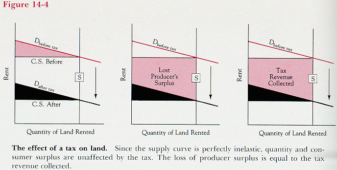
If the supply of land is perfectly inelastic, the supply curve for land is vertical, which implies that a tax on land, whether "paid" by owner or renter, is entirely borne by the owner, with none of it passed on to the renter. It also implies that a tax on land generates no excess burden--as you showed (I hope) in your answer to Problems 8 and 9 of Chapter 7. Both results are shown on Figure 14-4, where the tax is "paid" by the consumers. I drew it that way because a tax "paid" by the producer shifts the vertical supply curve vertically, which is difficult to show; the shifted curve would be identical to the unshifted one.

If you tax the market value of land, you discourage people from increasing the value of raw land by using capital and labor to improve it; the supply curve for improved land is by no means perfectly inelastic. So in order to impose the so-called single tax (a tax on the value of unimproved land, proposed as a substitute for all other taxes), you first have to find some way of estimating what the land would have been worth without any improvements--which is difficult.

Because land is the standard example of a good in perfectly inelastic supply and because payment for the use of land is called rent, the term rent has come to be used in economics in two different ways. One is to mean payment for the use of something, as distinguished from payment for ownership (price). In this sense, one buys cars from GM but rents them from Avis. The other is to mean payment for the use of something in fixed (i. e., perfectly inelastic) supply--or, more generally, to mean payments above what is needed to call something into existence.

In this second sense, rent can be applied to many things other than land. Scarce human talents--the abilities of an inventive genius or the combination of good coordination and very long legs--can be thought of as valuable resources in fixed supply and without close substitutes; the wages of Thomas Edison or Wilt Chamberlain may be analyzed as a sort of rent. Rent in this sense is a price that allocates the use of something among consumers but does not tell producers how much to produce, since the good is not being produced. The opposite case is payment for something with a horizontal supply curve--in that case, payment is simply equal to cost of production.

Just as one can argue for taxing away the rent on the site value of land, on the grounds that since land is in perfectly inelastic supply the tax will result in no excess burden, so one can argue for taxing away the rent on scarce human talents. Here again, problems arise when you try to identify what you want to tax. It is not clear how the IRS can tell which athletes and which inventors will continue to exercise their abilities even if they are paid no more than the normal market wage, and which will decide to do something else.

The shape of a supply curve depends on how much time producers have to adjust their output. In the very short run, practically everything is in fixed supply. In the longer run, many things are; and in the very long run, practically nothing is. One may even argue that if certain talents produce high incomes, the possessors of those talents will be rich and have lots of children, thus increasing the supply of those talents, or that a sufficiently high rent on land will encourage the exploration and development of other planets, thus increasing the quantity of land. So the economic analysis developed to explain the rent on land may be inapplicable to anything--even land--in the (very) long run. But it can be used to explain the behavior of many prices in the (sufficiently) short run--which may be a day for fresh fish and 30 years for houses.

In the previous chapter, I discussed goods whose cost of construction was a sunk cost, such as ships or factories. As long as the price shipowners get for carrying freight is high enough that their ships are worth something and not high enough to make it worth building more ships, the supply of ships is perfectly inelastic. The number of ships does not change with price, although it does gradually shrink as ships wear out. The same is true for prices at which it is worth building more ships--if we limit ourselves to times too short to build them. So the returns on ships can be thought of as a sort of rent--called a quasi-rent--provided we limit ourselves to a sufficiently short-term analysis. That is just what we did in Chapter 13.

The third factor of production is capital. The meanings of labor and of land (more generally, unproduced natural resources) seem fairly obvious; the meaning of capital is not. Does producing capital mean saving? Building factories? Investing your savings? What is capital--what does it look like?

One (good) answer is that using capital means using inputs now to produce outputs later. The more dollar-years required (number of dollars of inputs times number of years until the outputs appear--a slight oversimplification, since it ignores the effect of compound interest, but good enough for our purposes), the more the amount of capital used. Capital is productive because it is (often) possible to produce more output if you are willing to wait than if you are not--to spend a week chipping out a flint axe and then use the axe to cut down lots of trees instead of spending two days scraping through a tree with a chunk of unshaped flint, or to make machines to make machines to make machines to make cars instead of simply making cars. Capital is expensive because people usually prefer consumption now to consumption in the future and must be paid to give up the former in exchange for the latter. Capital goods are the physical objects (factories, machines, apple trees) produced by inputs now and used to produce outputs in the future.

The essential logic of the market for capital was described in Chapter 12, where we discussed the individual's decision of how much to borrow or save and the firm's decision of what investment projects were worth making. The higher the market interest rate, the more willing consumers are to give up consumption now in exchange for consumption in the future, since a higher interest rate means more future goods in exchange for a given quantity of present goods; so we expect the net supply of capital by consumers to increase with the interest rate--the supply curve slopes up. The higher the market interest rate, the lower the present value of a future stream of income, and thus the harder it is for an investment project to justify, in present value terms, its initial cost. So a higher interest rate means fewer investment projects that are worth making, and thus less money borrowed by firms--the demand curve slopes down. At some interest rate the two curves cross--the quantity consumers want to lend equals the quantity firms want to borrow. That is the market interest rate.

Describing capital as a single good is both less and more legitimate than is a similar simplification for land or labor. It is less legitimate because once capital goods are built, they are not very flexible; there is no way an automobile factory can produce steel or a milling machine grow grain. In the case of labor and land, we argued that one variety could substitute for another through a chain of intermediates--from secretary to ditchdigger in the one case, from wheat to soybeans in the other. Finding a chain to connect a steel mill to a drainage canal, or an invention (capital in the form of valuable knowledge produced by research) to a tractor, would be more difficult.

But treating all capital as one good is more legitimate than treating all labor or all land as one, if we consider capital before it is invested. A steel mill cannot be converted into a drainage canal--but an investor can decide whether he will use his savings to pay workers to build the one or the other. So the anticipated return on all investments--the interest rate--must be the same. If investors expected to make more by investing a dollar in building a steel mill than by investing a dollar in digging a drainage canal, capital would shift into steel; the increased supply of steel would drive down the price of steel and the return on investments in steel mills. The reduced supply of capital in canal building would, similarly, increase the return on investments in canals. Investors would continue to shift their capital out of the one use and into the other until the returns on the two were the same.

A reduction in the supply of steel mills--the destruction of a hundred mills by a war or an earthquake, say--will drive up the price of steel, increase the return on investments in steel mills, attract capital that would otherwise have gone elsewhere into the steel industry, and so drive up the general interest rate. Thus in the long run, there is a single quantity of capital and a single price for the use of capital--the interest rate. All capital is the same--before it is invested.

After it is invested, capital takes many forms. One of the most important is one that noneconomists rarely think of as capital--human capital. A medical student who invests $90,000 and six years in becoming a surgeon is bearing costs now in return for benefits in the future, just as he would be if he had invested his time and money in building a factory instead. If the salary of surgeons were not high enough to make investing in himself at least as attractive as investing in something else, he would have invested in physical capital instead. So the salary of a surgeon should be considered in part the wages of labor, in part the rent on certain scarce human talents, and in part interest on his human capital.

There is one important respect in which human capital differs from other forms of capital. If you have an idea for building a profitable factory but not enough money of your own to pay for it, you can raise more money either by letting other investors be part-owners of the factory or by borrowing, putting up the factory itself as your security. Your ability to invest in your own human capital is much more limited. You cannot sell shares of yourself because that would violate the laws against slavery--you cannot put yourself up as collateral for the same reason. You can borrow money to pay for your training--but after the money is spent, you may, if you wish, declare bankruptcy. Your creditors have no way of repossessing the training that you bought with their money.

In a market economy, investments in physical capital that can be expected to yield more than the normal market return will always be made. The same is not true for investments in human capital. They will be made only if the human in question (or his parents or someone else who values his future welfare or trusts him to pay back loans) can provide the necessary capital. In that respect, the market for human capital is an imperfect one.

The source of the imperfection was discussed in Chapter 12--insecure property rights. In Chapter 12, the property rights of owners of oil were insecure because of the possibility of expropriation--one consequence was to discourage investment in finding oil and drilling oil wells. Here the property rights of lenders are insecure because of the possibility of bankruptcy; the result is to discourage investment in (someone else's) human capital. The existence of this imperfection provides, on the one hand, an argument for government provision (or guarantees) of loans for education, and on the other hand, an argument for relaxing the prohibition against (self-chosen) slavery--to the extent of limiting the ability of people who borrow for their education to declare bankruptcy.

One respect in which factors differ is in the degree to which each is property. Land and physical capital are entirely property; they may be bought, sold, transferred, lent. Labor and human capital are property of a very limited sort, at least in our society. They may be rented out, but the contract can almost always be canceled at the will of the owner--the worker can always quit. Neither labor nor human capital can be sold, and neither can be used as collateral, since there is no way the lender can collect.

A second difference is in supply. Land is in absolutely fixed supply. Labor is also in fixed supply, if we include an individual's demand for his own labor (i.e. leisure) as part of demand rather than as something affecting supply. The quantity of labor changes over time because of changes in population; but since the producers of new labor (parents) do not own it and cannot sell it, it is not clear whether or not an increase in the price of labor will increase the supply, even in the long run. The quantity of capital changes as a result of saving; individuals who consume less than their income have the remainder available to invest. The higher the interest rate, the more you get next year in exchange for what you save this year, so we would expect the supply of new capital to increase with the interest rate--though for capital, as for labor, a backward-bending supply curve is not logically impossible.

We have now finished our sketch of the three factors of production. In ending, it is worth noting that there are some inputs to the productive process that do not fit comfortably into our categories. Two examples would be unproduced raw materials--iron ore, for instance--and special human abilities. Both behave like land, in the sense of being in fixed supply. But neither is land, since neither is a close substitute for the other things that are contained in the collection of related goods called land.

In Part 1 of this chapter, I showed how the distribution of income was determined and discussed how I might decide whether or not some particular change was in my interest by how it affected my share in the distribution. The conclusion was that I can expect to benefit by any change that raises the price of the productive inputs I sell or lowers the price of the goods I buy; I can expect to lose from any change that lowers the price of the inputs I sell or raises the price of the goods I buy.

The problem, as I pointed out at the time, is that many potential changes whose effects I might want to know cannot be evaluated in this way. They have no direct effect on the particular inputs I own and sell or the particular goods I consume, and the net consequence of their numerous indirect effects is hard to judge. The factors of production were introduced as a solution to this problem; when all inputs have been simplified down to three, it may be possible to judge both how some change affects each of the three factors and how a change in the prices of the factors affects my welfare.

That is what we will be doing in Part 3. We will consider three different public policy issues--immigration restrictions, limitations on foreign investment in poor countries, and governmental controls on land use. In each case, the question we are primarily interested in is not whether the policy is good or bad but who gains and who loses. In each case, we will try to answer that question by looking at the effect of the policy on the factors of production.

We can combine Parts 1 and 2 of this chapter in order to analyze a number of interesting questions; we will start with the effect of increased immigration on the welfare of the present inhabitants of the United States Prior to the 1920s, the United States followed a general policy of open immigration, except for some restrictions on immigration of Orientals. The result was a flood of immigrants that at its peak exceeded a million a year. Suppose we went back to open immigration. Who would benefit and who would lose?

Immigrants have, on average, less human and physical capital than the present inhabitants of the United States; they are less skilled and poorer. So one result of increased immigration would be an increase in the ratio of labor to capital in the United States Immigrants bring labor and some capital but no land, so another result would be to decrease the ratio of land to both labor and capital. Hence increased immigration would decrease the price of labor and increase the price of land; the effect on the price of capital is ambiguous, since it becomes scarcer relative to labor and less scarce relative to land. My guess is that since the additional immigrants who would come in under a policy of unrestricted immigration would bring very little capital with them--rich immigrants can come in under present laws--the return on capital would increase.

The net result would probably be to injure the most unskilled American workers. It might well benefit many or even most other workers, since what they are selling is not pure labor but a mixture containing a large amount of human capital. People who were net buyers of land would be injured by the increased price of land; people who were net sellers of land would be benefited. Net lenders would be benefited if the return on capital (the interest rate) increased; net borrowers would be injured.

Can we say anything about the overall effect on those presently living in the United States? Yes--but to do so, we must bring in arguments from a previous chapter. One way of looking at immigration restrictions is as barriers to trade; they prevent an American consumer from buying the labor of a Mexican worker by preventing the worker from coming to where the labor is wanted. The same comparative advantage arguments that were discussed in Chapter 6 and will be discussed again in Chapter 19 apply here as well. Since there is a net gain to trade, the abolition of immigration restrictions will produce a net benefit for present Americans, although some will be worse off--just as the abolition of tariffs produces a net benefit, although American auto workers (and GM stockholders) may be injured. These net benefits are in addition to the (very large) benefits to the new immigrants that are the reason they come.

Figure 14-5 shows the net effect of the immigration of Mexican carpenters discussed earlier; it corresponds to Figure 14-2 with the consumer and producer surpluses shown. Note that the darkly shaded area, representing the loss of producer surplus to existing carpenters, is included in, and therefore smaller than, the total shaded area (light and dark) representing the gain of consumer surplus to their customers. This implies that on net there is an increase in surplus even if we ignore the colored area, which represents the gain to the new immigrants.

---

---

A more precise discussion of what we mean by net benefits would carry us into the next chapter--which is about just such questions. A more rigorous explanation of why open immigration produces net benefits would carry us beyond the limits of this course. There are, however, two more points worth making before we finish with the question of immigration.

So far in my discussion of immigration, I have assumed a private property society in which the only way to get income is to sell labor or other inputs. In fact there are at least two other ways--from government (in the form of welfare, unemployment payments, and the like) and by private violation of property rights (theft and robbery). To the extent that new immigrants support themselves in those ways, they impose costs on the present inhabitants without providing corresponding benefits; in such a situation, the demonstration that new immigrants provide net benefits no longer holds.

It is unclear what, if any, connection there is between that argument and the abandonment of open immigration by the United States It is tempting to argue that immigration restrictions were one of the consequences of the welfare state. As long as it was clear that poor immigrants would have to support themselves, they were welcome; once they acquired the right to live off the taxes of those already here, they were not. The argument neatly links two of the major changes of the first half of this century--and does so in a way that fits nicely with my own ideological prejudices.

Unfortunately for the argument, immigration restrictions were imposed in the early 1920s, and the major increase in the size and responsibility of government occurred during the New Deal--about a decade later. At most one might conjecture that both resulted from the same changing view of the role of the state.

Whether or not there was any historical connection between the rise of the welfare state in the United States and the end of unrestricted immigration, it seems clear that present objections to immigrants often involve the fear that, as soon as they arrive, they will go on welfare. It is much less clear that that fear is justified; a good deal of evidence seems to suggest that new immigrants are more likely to start working their way up the income ladder--in response to the opportunity to earn what are, from the standpoint of many of them, phenomenally high wages.

My final comment on free immigration concerns its distributional effects. Opponents of immigration argue that it "hurts the poor and helps the rich," since the obvious losers are unskilled American workers. If we limit our discussion to those presently living here, they are probably right. But the big gainers from immigration would be the immigrants--most of whom are very much poorer than the American poor. From a national standpoint, free immigration may hurt the poor; from an international standpoint, it helps them. By world standards, the American poor are, if not rich, at least comfortably well off.

The term economic imperialism has at least two meanings. It is applied by some economists to the use of the economic approach to explain what are traditionally considered non-economic questions. We are imperialists trying to conquer the intellectual territory presently held by political scientists, sociologists, psychologists, and the like. Much more commonly, it is used by Marxists to describe--and attack--foreign investment in "developing" (i. e., poor) nations. The implication of the term is that such investment is only a subtler equivalent of military imperialism--a way by which capitalists in rich and powerful countries control and exploit the inhabitants of poor and weak countries.

There is one interesting feature of such "economic imperialism" that seems to have escaped the notice of most of those who use the term. Developing countries are generally labor rich and capital poor; developed countries are, relatively, capital rich and labor poor. One result is that in developing countries, the return on labor is low and the return on capital is high--wages are low and profits high. That is why they are attractive to foreign investors.

To the extent that foreign investment occurs, it raises the amount of capital in the country, driving wages up and profits down. The effect is exactly analogous to the effect of free migration. If people move from labor-rich countries to labor-poor ones, they drive wages down and rents and profits up in the countries they go to, while having the opposite effect in the countries they come from. If capital moves from capital-rich countries to capital-poor ones, it drives profits down and wages up in the countries it goes to and has the opposite effect in the countries it comes from.

The people who attack "economic imperialism" generally regard themselves as champions of the poor and oppressed. To the extent that they succeed in preventing foreign investment in poor countries, they are benefiting the capitalists of those countries by holding up profits and injuring the workers by holding down wages. It would be interesting to know how much of the clamor against foreign investment in such countries is due to Marxist ideologues who do not understand this and how much is financed by local capitalists who do.

I should warn you that in the last few paragraphs I have used the term profit in the conventional sense of the return to capital, that being the way it is usually used in such discussions. A better term would be interest. That way, one avoids confusing profit in the sense of the return on capital with profit in the sense of economic profit--revenue minus all costs, including the cost of capital.

In the United States and in similar societies elsewhere, there are often extensive limitations on how property owners can use their land. Many of these limitations can be defended in terms of externalities--a subject that will be discussed in Chapter 18. Whether or not the restrictions are justified, it is interesting to analyze their distributional effects.

Suppose the English government requires (as it does) that "greenbelts" be established around major cities--areas surrounding the urban center within which dense populations are prohibited. The result is to reduce the total amount of residential land available in such cities. The result of that is to increase rents. A law that is defended as a way of protecting urban beauty against greedy developers has as one of its effects raising the income of urban landlords at the expense of their tenants. It would be interesting to analyze the sources of support for imposing and maintaining greenbelt legislation, in order to see how much comes from the residents whose environment the legislation claims to protect and how much from the landlords whose income it increases.

So far, we have been using the ideas of Parts 1 and 2 of this chapter to determine who is injured or benefited by various policies. The same ideas can also be used to answer another question: What determines the different wages in different professions?

We begin with the observation from Part 2 that in equilibrium all sorts of labor are in some sense the same, as are all sorts of capital and land. If so, then one would expect that all jobs would receive the same pay. Obviously this is not so. Why?

The first answer is that we may not be in long-run equilibrium. Equilibrium is created and maintained by the fact that when one profession is more attractive than another, people tend to leave the less attractive profession and enter the more attractive one and new workers coming onto the market tend to enter the more attractive profession. As workers enter the attractive professions, they drive down their wages; as workers leave the unattractive ones, the wages in those professions rise. The process stops only when all professions are equally attractive.

All of this takes time. An individual who has spent considerable time and money training himself for one profession will switch to another only if the return is not only larger but large enough to justify the cost of the move. This is less of a problem for new workers coming onto the market, since they have not yet made the investment--but it may take a long time before the reduced inflow of new workers has much effect on the total number in the profession. So if an unexpected reduction in the demand for some particular type of labor pushes wages in that field below their long-run equilibrium level, it may be years before they come all the way back up. Similarly, an unexpected increase in demand for some particular sort of labor may keep wages above the normal level for some time, especially if the profession is one that requires lengthy training. The logic of the situation is essentially the same as in Chapter 13, applied to people instead of ships.

A second answer is that differing wages may reflect differing abilities. If, for example, intelligence is useful in practically any field and if nuclear physicists are, on average, more intelligent than grocery store clerks, then they will also have higher wages. The individual nuclear physicist may, in this case, earn no more than he would if he were a clerk--but the same man who is an average physicist, earning an average physicist's salary, would be an above-average clerk, earning an above-average clerk's salary. This is the case I described earlier as one person "containing more labor" than another. One hour of the intelligent worker's time may be equivalent to two hours of the average worker's time.

If this were the whole story, there is no obvious reason why nuclear physicists would be more intelligent than clerks--the intelligent individual would get the same return in either profession. In fact, of course, intelligence--and other abilities--are more useful in some fields than in others. Being seven feet tall is very useful if you are a basketball player; if you are a college professor, it merely means that you bump your head a lot.

Differences in such specialized abilities may not matter very much if the abilities are in sufficiently large supply. If 10 percent of the population consisted of men who were seven feet tall and well coordinated, basketball players would not get unusually high salaries--there would be too many tall clerks, tall professors, and tall ditchdiggers willing to enter the profession if they did. Similarly, whether the talents that make a good salesman bring high salaries to their possessors depends on both the supply of and demand for those talents. If equilibrium is reached only when all of the people who have those talents, plus some of those who do not have them, are salesmen, then the return to selling must be high enough to make it a reasonably attractive profession even to those who are not unusually talented at it--and a very attractive profession to those who are. If, on the other hand, in equilibrium all of the salesmen are talented and only some of those with the appropriate talents are salesmen, then talented salesmen will receive only a normal return for their efforts.

The logic of the situation is the same as in our earlier discussion of growing wheat and soybeans. Figures 14-6a and b show the argument in graphical form. On Figure 14-6a the number of tall people (Q_tall) is more than enough to bring the wages of basketball players down to the wages of other jobs, so all jobs receive the same wage (W). On figure 14-6b basketball has become more popular; the demand for basketball players (D_bball) has increased to the point where even with all the tall people playing basketball, their wage (W_t) is above the wage for other jobs (W_o).

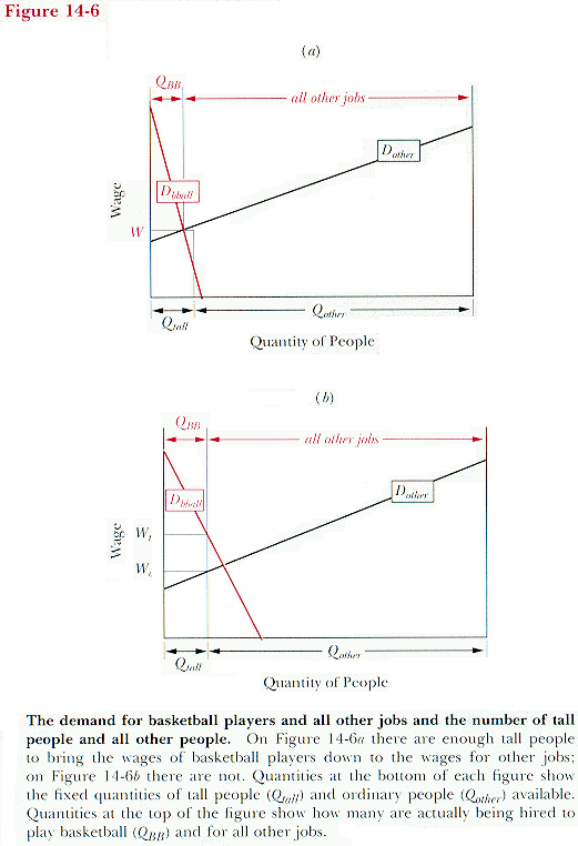
Usually, the situation is not quite that extreme. There are people who could play basketball and do not; but they are, on average, shorter (or worse coordinated or in some other way less suited for basketball) than the people who do play. In equilibrium the wage is such that the marginal basketball player--the individual just balanced between choosing to play basketball and choosing to do something else--finds both alternatives equally attractive. If the average player is considerably better than the marginal one, he will also receive a higher salary. The same argument can be worked through for any profession in which the individual's productivity depends on his possession of scarce characteristics or abilities.

We have now discussed two reasons why different professions might not, on net, be equally attractive--disequilibrium and differential abilities. There remains the possibility that even if neither of those factors is important--even if all professions are equally attractive--they may still be attractive in different ways.

Consider a group of professions. We assume that none of them requires any special human abilities; indeed, to make the situation even simpler, we assume that all individuals start with the same abilities. We also assume that the economy is in equilibrium; there have been no unexpected changes in the demand for different sorts of labor, so everyone is getting about the wage he expected to get when he chose his field.

Even in this situation, we may observe wide variations in the wages received by people in different professions. What is equal in equilibrium is the net advantage in each field, not the wage. If, for example, a particular profession, such as economics, is much more fun than other professions, it will also pay less. If it did not--if its wages were the same as those in less enjoyable fields--then on net it would be more attractive. People who were leading dull lives as ditchdiggers, sociologists, or lawyers would pour into the field, driving down the wage.

The argument applies not only to professions that are more fun but also to professions that have other nonpecuniary advantages. If, for example, many people want to be film or rock stars, not because the job is fun but because they like the idea of being watched by adoring multitudes, that will tend to drive down the wages of those professions. The same argument also works in reverse, for professions that have nonpecuniary disadvantages. That is why it costs more to hire people to drive trucks loaded with dynamite than trucks loaded with dirt.

A second factor that makes wages unequal even when net advantage is equal is the difference in the cost of entering different professions. Becoming a checkout clerk requires almost no training; becoming an actuary requires years of study. If both professions earned the same wages, few people would become actuaries. In equilibrium the wage of the actuary must be enough higher to repay the time and expense invested in learning the job. Since the cost of training occurs at the beginning of his career and the return occurs later, the actuary must receive enough extra income to pay not only the cost of his training but also the interest on his investment in himself. If he did not, he would be better off investing his money in something other than himself and becoming a clerk instead. The wages of actuaries must pay for their human capital as well as their raw labor.

There is one more element that should be taken into account in explaining wage differentials--uncertainty. In some professions, the wage is fairly predictable; in others it is not. Movie stars make very large incomes, but the only actress I ever knew personally supported herself largely by temporary secretarial work. In a profession where most people are failures, at least from a financial standpoint, it is not surprising that the few successes do very well. An individual entering such a profession is, in effect, buying a ticket in a lottery--one chance of making several hundred thousand dollars a year, 999 chances of barely scraping by on an occasional acting job supplemented by part-time work and unemployment compensation, and a few chances of something in between the two extremes. My impression is that the average wage of actors and actresses is quite low and that the willingness of men and women to enter the profession reflects either unrealistic optimism, large nonpecuniary returns from doing what they really want to do, or both.

1. Suppose you wanted to calculate the Gini coefficient properly; further suppose you had complete information about everyone's income from birth to death. Exactly how would you solve the problem (confusion of changing income over time with changing income across people) discussed at the beginning of this chapter? (Hint: Use a concept from Chapter 12.)

2. The chapter discusses ways in which one might try to justify the distribution of income produced by a market. What do you believe is a just distribution? What should determine who gets how much?

3. Why is a backward-bending supply curve more plausible for labor considered as a factor of production than for any particular kind of labor (table making) or the product of such labor?

4. My wife is a geologist employed by an oil company. We spend less than one percent of our joint income for gasoline and several percent more for heating (gas) and power. Do you think we are better or worse off if the price of oil goes up? Would your answer be very much different if we had oil heat? If she was a geologist employed by a university? Discuss.

5. The government decides there are too many buildings in America and proposes a 50 percent tax on constructing new buildings. Which of the following groups will support the tax? Which will oppose it? Why?

a. Investors who own buildings. b. Building contractors. c. Tenants. d. Landlords. e. Owners of undeveloped land.

6. What alternative professions would you seriously consider entering if their wage, relative to the wage you expect in the profession you plan to follow, rose by 10 percent? By 50 percent? What alternative professions would you have seriously considered if, before you started training for this one, their wages had been 10 percent higher than they were? If they had been 50 percent higher?

7. Suppose we say that two professions are linked if there is at least one person in each who would have been in the other if the wage had been 10 percent higher. How many steps does it take to link your profession to the profession of a ditchdigger? A professional athlete? A hit man? A brain surgeon? A homemaker? Describe plausible chains in each case.

(Example: The chain economist-lawyer-politician links me to a politician and has two links. Some economists are people who might well have become lawyers instead--and would have if the wages of lawyers were a little higher. Some lawyers are people who might well have become politicians instead--and would have if the "wages" of politicians were a little higher.)

8. Explain briefly why Problems 6 and 7 are in this chapter.

9. The concern with population questions in recent decades has been fueled in part by the belief that poor countries are poor mainly because they are overpopulated. Look up population densities (people per square mile) and income figures for China, Japan, India, West Germany, Belgium, Taiwan, and Mexico. Does it look as though poverty is mainly a function of population density? Looking at other countries, does the conclusion suggested by these cases seem to be typical? Discuss.

10. There are some people who very much want to be actors and will enter the profession even if they receive barely enough to live on. Discuss, as precisely as possible, under what circumstances actors will make barely enough to live on, under what circumstances they will make about the same wages as people in other fields, and under what circumstances they will make more. You may wish to simplify the problem by ignoring the probabilistic element--assume all actors make the same amount. You may find it useful to consider the effect on wages of different possible supply and demand curves for actors.

11. We described the additional salary received by someone who possesses scarce human talents as a sort of rent. What similar term might be used to describe the additional salary received by someone in a profession where wages are temporarily above their long-run equilibrium? Discuss.

The classic discussion of the economics of wage differentials was published in 1776. It can be found in Chapter X, Book I, of Adam Smith, An Inquiry into the Nature and Causes of the Wealth of Nations (New York: Oxford University Press, 1976). The book is still well worth reading.

Students interested in a much more advanced treatment of one of the subjects raised in this chapter may want to look at Gary Becker, Human Capital: A Theoretical and Empirical Analysis (2nd ed; New York: Columbia University Press, 1975).

The most famous supporter of the idea of taxing the site value of land, Henry George, stated his argument in Progress and Poverty (New York: Robert Schalkenbach Foundation, 1984).